Section 6.1 : Exponential Functions
Let’s start off this section with the definition of an exponential function.
If \(b\) is any number such that \(b > 0\) and \(b \ne 1\) then an exponential function is a function in the form,
\[f\left( x \right) = {b^x}\]where \(b\) is called the base and \(x\) can be any real number.
Notice that the \(x\) is now in the exponent and the base is a fixed number. This is exactly the opposite from what we’ve seen to this point. To this point the base has been the variable, \(x\) in most cases, and the exponent was a fixed number. However, despite these differences these functions evaluate in exactly the same way as those that we are used to. We will see some examples of exponential functions shortly.
Before we get too far into this section we should address the restrictions on \(b\). We avoid one and zero because in this case the function would be,
\[f\left( x \right) = {0^x} = 0\hspace{0.25in}{\mbox{and}}\hspace{0.25in}\,\,\,\,\,f\left( x \right) = {1^x} = 1\]and these are constant functions and won’t have many of the same properties that general exponential functions have.
Next, we avoid negative numbers so that we don’t get any complex values out of the function evaluation. For instance, if we allowed \(b = - 4\) the function would be,
\[f\left( x \right) = {\left( { - 4} \right)^x}\hspace{0.25in} \Rightarrow \,\hspace{0.25in}\,\,\,\,f\left( {\frac{1}{2}} \right) = {\left( { - 4} \right)^{\frac{1}{2}}} = \sqrt { - 4} \]and as you can see there are some function evaluations that will give complex numbers. We only want real numbers to arise from function evaluation and so to make sure of this we require that \(b\) not be a negative number.
Now, let’s take a look at a couple of graphs. We will be able to get most of the properties of exponential functions from these graphs.
Okay, since we don’t have any knowledge on what these graphs look like we’re going to have to pick some values of \(x\) and do some function evaluations. Function evaluation with exponential functions works in exactly the same manner that all function evaluation has worked to this point. Whatever is in the parenthesis on the left we substitute into all the \(x\)’s on the right side.
Here are some evaluations for these two functions,
| \(x\) | \(f\left( x \right) = {2^x}\) | \(g\left( x \right) = {\left( {\frac{1}{2}} \right)^x}\) |
|---|---|---|
| -2 | \(f\left( { - 2} \right) = {2^{ - 2}} = \frac{1}{{{2^2}}} = \frac{1}{4}\) | \(g\left( { - 2} \right) = {\left( {\frac{1}{2}} \right)^{ - 2}} = {\left( {\frac{2}{1}} \right)^2} = 4\) |
| -1 | \(f\left( { - 1} \right) = {2^{ - 1}} = \frac{1}{{{2^1}}} = \frac{1}{2}\) | \(g\left( { - 1} \right) = {\left( {\frac{1}{2}} \right)^{ - 1}} = {\left( {\frac{2}{1}} \right)^1} = 2\) |
| 0 | \(f\left( 0 \right) = {2^0} = 1\) | \(g\left( 0 \right) = {\left( {\frac{1}{2}} \right)^0} = 1\) |
| 1 | \(f\left( 1 \right) = {2^1} = 2\) | \(g\left( 1 \right) = {\left( {\frac{1}{2}} \right)^1} = \frac{1}{2}\) |
| 2 | \(f\left( 2 \right) = {2^2} = 4\) | \(g\left( 2 \right) = {\left( {\frac{1}{2}} \right)^2} = \frac{1}{4}\) |
Here is the sketch of the two graphs.
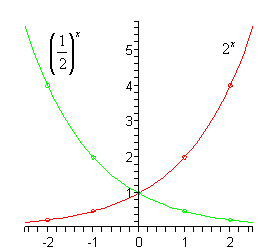
Note as well that we could have written \(g\left( x \right)\) in the following way,
\[g\left( x \right) = {\left( {\frac{1}{2}} \right)^x} = \frac{1}{{{2^x}}} = {2^{ - x}}\]Sometimes we’ll see this kind of exponential function and so it’s important to be able to go between these two forms.
Now, let’s talk about some of the properties of exponential functions.
Properties of \(f\left( x \right) = {b^x}\)
- The graph of \(f\left( x \right)\) will always contain the point \(\left( {0,1} \right)\). Or put another way, \(f\left( 0 \right) = 1\) regardless of the value of \(b\).
- For every possible \(b\) we have \({b^x} > 0\). Note that this implies that \({b^x} \ne 0\).
- If \(0 < b < 1\) then the graph of \({b^x}\) will decrease as we move from left to right. Check out the graph of \({\left( {\frac{1}{2}} \right)^x}\) above for verification of this property.
- If \(b > 1\) then the graph of \({b^x}\) will increase as we move from left to right. Check out the graph of \({2^x}\) above for verification of this property.
- If \({b^x} = {b^y}\) then \(x = y\)
All of these properties except the final one can be verified easily from the graphs in the first example. We will hold off discussing the final property for a couple of sections where we will actually be using it.
As a final topic in this section we need to discuss a special exponential function. In fact this is so special that for many people this is THE exponential function. Here it is,
\[f\left( x \right) = {{\bf{e}}^x}\]where \({\bf{e}} = 2.718281828 \ldots \). Note the difference between \(f\left( x \right) = {b^x}\) and \(f\left( x \right) = {{\bf{e}}^x}\). In the first case \(b\) is any number that meets the restrictions given above while e is a very specific number. Also note that e is not a terminating decimal.
This special exponential function is very important and arises naturally in many areas. As noted above, this function arises so often that many people will think of this function if you talk about exponential functions. We will see some of the applications of this function in the final section of this chapter.
Let’s get a quick graph of this function.
Let’s first build up a table of values for this function.
| \(x\) | -2 | -1 | 0 | 1 | 2 |
| \(f(x)\) | 0.1353… | 0.3679… | 1 | 2.718… | 7.389… |
To get these evaluation (with the exception of \(x = 0\)) you will need to use a calculator. In fact, that is part of the point of this example. Make sure that you can run your calculator and verify these numbers.
Here is a sketch of this graph.
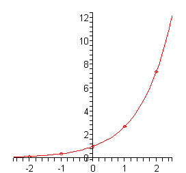
Notice that this is an increasing graph as we should expect since \({\bf{e}} = 2.718281827 \ldots > 1\).
There is one final example that we need to work before moving onto the next section. This example is more about the evaluation process for exponential functions than the graphing process. We need to be very careful with the evaluation of exponential functions.
Here is a quick table of values for this function.
| \(x\) | -1 | 0 | 1 | 2 | 3 |
| >\(g(x)\) | 32.945… | 9.591… | 1 | -2.161… | -3.323… |
Now, as we stated above this example was more about the evaluation process than the graph so let’s go through the first one to make sure that you can do these.
\[\begin{align*}g\left( { - 1} \right) & = 5{{\bf{e}}^{1 - \left( { - 1} \right)}} - 4\\ & = 5{{\bf{e}}^2} - 4\\ & = 5\left( {7.389} \right) - 4\end{align*}\]Notice that when evaluating exponential functions we first need to actually do the exponentiation before we multiply by any coefficients (5 in this case). Also, we used only 3 decimal places here since we are only graphing. In many applications we will want to use far more decimal places in these computations.
Here is a sketch of the graph.
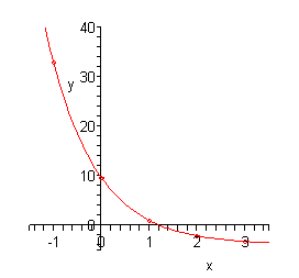
Notice that this graph violates all the properties we listed above. That is okay. Those properties are only valid for functions in the form \(f\left( x \right) = {b^x}\) or \(f\left( x \right) = {{\bf{e}}^x}\). We’ve got a lot more going on in this function and so the properties, as written above, won’t hold for this function.