Section 4.11 : Linear Approximations
In this section we’re going to take a look at an application not of derivatives but of the tangent line to a function. Of course, to get the tangent line we do need to take derivatives, so in some way this is an application of derivatives as well.
Given a function, \(f\left( x \right)\), we can find its tangent at \(x = a\). The equation of the tangent line, which we’ll call \(L\left( x \right)\) for this discussion, is,
\[L\left( x \right) = f\left( a \right) + f'\left( a \right)\left( {x - a} \right)\]Take a look at the following graph of a function and its tangent line.
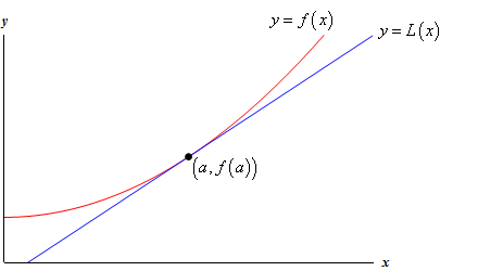
From this graph we can see that near \(x = a\) the tangent line and the function have nearly the same graph. On occasion we will use the tangent line, \(L\left( x \right)\), as an approximation to the function, \(f\left( x \right)\), near \(x = a\). In these cases we call the tangent line the linear approximation to the function at \(x = a\).
So, why would we do this? Let’s take a look at an example.
Since this is just the tangent line there really isn’t a whole lot to finding the linear approximation.
\[f'\left( x \right) = \frac{1}{3}{x^{ - \frac{2}{3}}} = \frac{1}{{3\,\sqrt[3]{{{x^2}}}}}\hspace{0.5in}f\left( 8 \right) = 2\hspace{0.25in}f'\left( 8 \right) = \frac{1}{{12}}\]The linear approximation is then,
\[L\left( x \right) = 2 + \frac{1}{{12}}\left( {x - 8} \right) = \frac{1}{{12}}x + \frac{4}{3}\]Now, the approximations are nothing more than plugging the given values of \(x\) into the linear approximation. For comparison purposes we’ll also compute the exact values.
\[\begin{align*}L\left( {8.05} \right) & = 2.00416667 & \hspace{0.75in} \sqrt[3]{{8.05}} & = 2.00415802\\ L\left( {25} \right) & = 3.41666667 & \hspace{0.75in} \sqrt[3]{{25}} & = 2.92401774\end{align*}\]So, at \(x = 8.05\) this linear approximation does a very good job of approximating the actual value. However, at \(x = 25\) it doesn’t do such a good job.
This shouldn’t be too surprising if you think about it. Near \(x = 8\) both the function and the linear approximation have nearly the same slope and since they both pass through the point \(\left( {8,2} \right)\) they should have nearly the same value as long as we stay close to \(x = 8\). However, as we move away from \(x = 8\) the linear approximation is a line and so will always have the same slope while the function’s slope will change as \(x\) changes and so the function will, in all likelihood, move away from the linear approximation.
Here’s a quick sketch of the function and its linear approximation at \(x = 8\).
![This is a graph of $f\left( x \right)=\sqrt[3]{x}$. Also shown on the graph is the tangent line to this graph at the point (8,2). The tangent line falls above the graph of the function.](LinearApproximations_Files/image002.png)
As noted above, the farther from \(x = 8\) we get the more distance separates the function itself and its linear approximation.
Linear approximations do a very good job of approximating values of \(f\left( x \right)\) as long as we stay “near” \(x = a\). However, the farther away from \(x = a\) we get the worse the approximation is liable to be. The main problem here is that how near we need to stay to \(x = a\) in order to get a good approximation will depend upon both the function we’re using and the value of \(x = a\) that we’re using. Also, there will often be no easy way of predicting how far away from \(x = a\) we can get and still have a “good” approximation.
Let’s take a look at another example that is actually used fairly heavily in some places.
Again, there really isn’t a whole lot to this example. All that we need to do is compute the tangent line to \(\sin \theta \) at \(\theta = 0\).
\[\begin{align*}f\left( \theta \right) & = \sin \theta & \hspace{0.75in} f'\left( \theta \right) & = \cos \theta \\ f\left( 0 \right) & = 0 & \hspace{0.75in}f'\left( 0 \right) & = 1\end{align*}\]The linear approximation is,
\[\begin{align*}L\left( \theta \right) & = f\left( 0 \right) + f'\left( 0 \right)\left( {\theta - a} \right)\\ & = 0 + \left( 1 \right)\left( {\theta - 0} \right)\\ & = \theta \end{align*}\]So, as long as \(\theta \) stays small we can say that \(\sin \theta \approx \theta \).
This is actually a somewhat important linear approximation. In optics this linear approximation is often used to simplify formulas. This linear approximation is also used to help describe the motion of a pendulum and vibrations in a string.