Section 15.4 : Double Integrals in Polar Coordinates
To this point we’ve seen quite a few double integrals. However, in every case we’ve seen to this point the region \(D\) could be easily described in terms of simple functions in Cartesian coordinates. In this section we want to look at some regions that are much easier to describe in terms of polar coordinates. For instance, we might have a region that is a disk, ring, or a portion of a disk or ring. In these cases, using Cartesian coordinates could be somewhat cumbersome. For instance, let’s suppose we wanted to do the following integral,
\[\iint\limits_{D}{{f\left( {x,y} \right)\,dA}},\,\,\,\,\,D{\mbox{ is the disk of radius 2}}\]To this we would have to determine a set of inequalities for \(x\) and \(y\) that describe this region. These would be,
\[\begin{array}{c} - 2 \le x \le 2\\ - \sqrt {4 - {x^2}} \le y \le \sqrt {4 - {x^2}} \end{array}\]With these limits the integral would become,
\[\iint\limits_{D}{{f\left( {x,y} \right)\,dA}} = \int_{{\, - 2}}^{{\,2}}{{\int_{{ - \sqrt {4 - {x^2}} }}^{{\,\sqrt {4 - {x^2}} }}{{f\left( {x,y} \right)\,dy}}\,dx}}\]Due to the limits on the inner integral this is liable to be an unpleasant integral to compute.
However, a disk of radius 2 can be defined in polar coordinates by the following inequalities,
\[\begin{array}{c}0 \le \theta \le 2\pi \\ 0 \le r \le 2\end{array}\]These are very simple limits and, in fact, are constant limits of integration which almost always makes integrals somewhat easier.
So, if we could convert our double integral formula into one involving polar coordinates we would be in pretty good shape. The problem is that we can’t just convert the \(dx\) and the \(dy\) into a \(dr\) and a \(d\theta \). In computing double integrals to this point we have been using the fact that \(dA = dx\,dy\) and this really does require Cartesian coordinates to use. Once we’ve moved into polar coordinates \(dA \ne dr\,d\theta \) and so we’re going to need to determine just what \(dA\) is under polar coordinates.
So, let’s step back a little bit and start off with a general region in terms of polar coordinates and see what we can do with that. Here is a sketch of some region using polar coordinates.
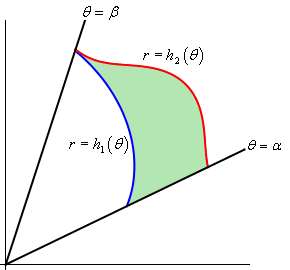
So, our general region will be defined by inequalities,
\[\begin{array}{c}\alpha \le \theta \le \beta \\ {h_1}\left( \theta \right) \le r \le {h_2}\left( \theta \right)\end{array}\]Now, to find \(dA\) let’s redo the figure above as follows,
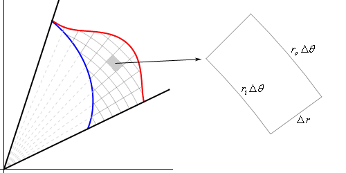
As shown, we’ll break up the region into a mesh of radial lines and arcs. Now, if we pull one of the pieces of the mesh out as shown we have something that is almost, but not quite a rectangle. The area of this piece is \(\Delta A\). The two sides of this piece both have length \(\Delta \,r = {r_o} - {r_i}\) where \({r_o}\) is the radius of the outer arc and \({r_i}\) is the radius of the inner arc. Basic geometry then tells us that the length of the inner edge is \({r_i}\,\Delta \,\theta \) while the length of the out edge is \({r_o}\,\Delta \,\theta \) where \(\Delta \,\theta \) is the angle between the two radial lines that form the sides of this piece.
Now, let’s assume that we’ve taken the mesh so small that we can assume that \({r_i} \approx {r_o} = r\) and with this assumption we can also assume that our piece is close enough to a rectangle that we can also then assume that,
\[\Delta A \approx r\,\Delta \,\theta \,\Delta \,r\]Also, if we assume that the mesh is small enough then we can also assume that,
\[dA \approx \Delta A\hspace{0.5in}d\theta \approx \Delta \theta \hspace{0.5in}dr \approx \Delta \,r\]With these assumptions we then get \(dA \approx r\,dr\,d\theta \).
In order to arrive at this we had to make the assumption that the mesh was very small. This is not an unreasonable assumption. Recall that the definition of a double integral is in terms of two limits and as limits go to infinity the mesh size of the region will get smaller and smaller. In fact, as the mesh size gets smaller and smaller the formula above becomes more and more accurate and so we can say that,
We’ll see another way of deriving this once we reach the Change of Variables section later in this chapter. This second way will not involve any assumptions either and so it maybe a little better way of deriving this.
Before moving on it is again important to note that \(dA \ne dr\,d\theta \). The actual formula for \(dA\) has an \(r\) in it. It will be easy to forget this \(r\) on occasion, but as you’ll see without it some integrals will not be possible to do.
Now, if we’re going to be converting an integral in Cartesian coordinates into an integral in polar coordinates we are going to have to make sure that we’ve also converted all the \(x\)’s and \(y\)’s into polar coordinates as well. To do this we’ll need to remember the following conversion formulas,
\[x = r\cos \theta \hspace{0.5in}y = r\sin \theta \hspace{0.5in}{r^2} = {x^2} + {y^2}\]We are now ready to write down a formula for the double integral in terms of polar coordinates.
It is important to not forget the added \(r\) and don’t forget to convert the Cartesian coordinates in the function over to polar coordinates.
Let’s look at a couple of examples of these kinds of integrals.
- \(\displaystyle \iint\limits_{D}{{2x\,y\,dA}}\), \(D\) is the portion of the region between the circles of radius 2 and radius 5 centered at the origin that lies in the first quadrant.
- \(\displaystyle \iint\limits_{D}{{{{\bf{e}}^{{x^2} + {y^2}}}\,dA}}\), \(D\) is the unit disk centered at the origin.
First let’s get \(D\) in terms of polar coordinates. The circle of radius 2 is given by \(r = 2\) and the circle of radius 5 is given by \(r = 5\). We want the region between the two circles, so we will have the following inequality for \(r\).
\[2 \le r \le 5\]Also, since we only want the portion that is in the first quadrant we get the following range of \(\theta \)’s.
\[0 \le \theta \le \frac{\pi }{2}\]Now that we’ve got these we can do the integral.
\[\iint\limits_{D}{{2x\,y\,dA}} = \int_{{\,0}}^{{\,\frac{\pi }{2}}}{{\int_{{\,2}}^{{\,5}}{{2\left( {r\cos \theta } \right)\left( {r\sin \theta } \right)r\,dr}}\,d\theta }}\]Don’t forget to do the conversions and to add in the extra \(r\). Now, let’s simplify and make use of the double angle formula for sine to make the integral a little easier.
\[\begin{align*}\iint\limits_{D}{{2x\,y\,dA}} & = \int_{{\,0}}^{{\,\frac{\pi }{2}}}{{\int_{{\,2}}^{{\,5}}{{{r^3}\sin \left( {2\theta } \right)\,dr}}\,d\theta }}\\ & = \int_{{\,0}}^{{\,\frac{\pi }{2}}}{{\left. {\frac{1}{4}{r^4}\sin \left( {2\theta } \right)} \right|_2^5\,d\theta }}\\ & = \int_{{\,0}}^{{\,\frac{\pi }{2}}}{{\frac{{609}}{4}\sin \left( {2\theta } \right)\,d\theta }}\\ & = \left. { - \frac{{609}}{8}\cos \left( {2\theta } \right)} \right|_0^{\frac{\pi }{2}}\\ & = \frac{{609}}{4}\end{align*}\]b \(\displaystyle \iint\limits_{D}{{{{\bf{e}}^{{x^2} + {y^2}}}\,dA}}\), \(D\) is the unit disk centered at the origin. Show Solution
In this case we can’t do this integral in terms of Cartesian coordinates. We will however be able to do it in polar coordinates. First, the region \(D\) is defined by,
\[\begin{array}{c}0 \le \theta \le 2\pi \\ 0 \le r \le 1\end{array}\]In terms of polar coordinates the integral is then,
\[\iint\limits_{D}{{{{\bf{e}}^{{x^2} + {y^2}}}\,dA}} = \int_{{\,0}}^{{\,2\pi }}{{\int_{{\,0}}^{{\,1}}{{r\,{{\bf{e}}^{{r^2}}}\,dr}}\,d\theta }}\]Notice that the addition of the \(r\) gives us an integral that we can now do. Here is the work for this integral.
\[\begin{align*}\iint\limits_{D}{{{{\bf{e}}^{{x^2} + {y^2}}}\,dA}} & = \int_{{\,0}}^{{\,2\pi }}{{\int_{{\,0}}^{{\,1}}{{r\,{{\bf{e}}^{{r^2}}}\,dr}}\,d\theta }}\\ & = \int_{{\,0}}^{{\,2\pi }}{{\left. {\frac{1}{2}{{\bf{e}}^{{r^2}}}} \right|_0^1\,d\theta }}\\ & = \int_{{\,0}}^{{\,2\pi }}{{\frac{1}{2}\left( {{\bf{e}} - 1} \right)\,d\theta }}\\ & = \pi \left( {{\bf{e}} - 1} \right)\end{align*}\]Let’s not forget that we still have the two geometric interpretations for these integrals as well.
Here is a sketch of the region, \(D\), that we want to determine the area of.
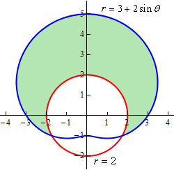
To determine this area we’ll need to know that value of \(\theta\) for which the two curves intersect. We can determine these points by setting the two equations equal and solving.
\[\begin{align*}3 + 2\sin \theta & = 2\\ \sin \theta & = - \frac{1}{2}\hspace{0.5in} \Rightarrow \hspace{0.5in}\theta = \frac{{7\pi }}{6},\frac{{11\pi }}{6}\end{align*}\]Here is a sketch of the figure with these angles added.
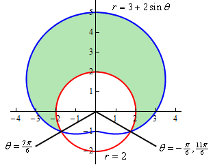
Note as well that we’ve acknowledged that \( - \frac{\pi }{6}\) is another representation for the angle \(\frac{{11\pi }}{6}\). This is important since we need the range of \(\theta\) to actually enclose the regions as we increase from the lower limit to the upper limit. If we’d chosen to use \(\frac{{11\pi }}{6}\) then as we increase from \(\frac{{7\pi }}{6}\) to \(\frac{{11\pi }}{6}\) we would be tracing out the lower portion of the circle and that is not the region that we are after.
So, here are the ranges that will define the region.
\[\begin{array}{c}\displaystyle - \frac{\pi }{6} \le \theta \le \frac{{7\pi }}{6}\\ 2 \le r \le 3 + 2\sin \theta \end{array}\]To get the ranges for \(r\) the function that is closest to the origin is the lower bound and the function that is farthest from the origin is the upper bound.
The area of the region \(D\) is then,
\[\begin{align*}A &= \iint\limits_{D}{{dA}}\\ & = \int_{{ - {\pi }/{6}\;}}^{{\,7{\pi }/{6}\;}}{{\int_{2}^{{3 + 2\sin \theta }}{{r\,drd\theta }}}}\\ & = \int_{{ - {\pi }/{6}\;}}^{{\,7{\pi }/{6}\;}}{{\left. {\frac{1}{2}{r^2}} \right|_2^{3 + 2\sin \theta }\,d\theta }}\\ & = \int_{{ - {\pi }/{6}\;}}^{{\,7{\pi }/{6}\;}}{{\frac{5}{2} + 6\sin \theta + 2{{\sin }^2}\theta \,d\theta }}\\ & = \int_{{ - {\pi }/{6}\;}}^{{\,7{\pi }/{6}\;}}{{\frac{7}{2} + 6\sin \theta - \cos \left( {2\theta } \right)\,d\theta }}\\ & = \left. {\left( {\frac{7}{2}\theta - 6\cos \theta - \frac{1}{2}\sin \left( {2\theta } \right)} \right)} \right|_{ - \frac{\pi }{6}}^{\frac{{7\pi }}{6}}\\ & = \frac{{11\sqrt 3 }}{2} + \frac{{14\pi }}{3} = 24.187\end{align*}\]We know that the formula for finding the volume of a region is,
\[V = \iint\limits_{D}{{f\left( {x,y} \right)\,dA}}\]In order to make use of this formula we’re going to need to determine the function that we should be integrating and the region \(D\) that we’re going to be integrating over.
The function isn’t too bad. It’s just the sphere, however, we do need it to be in the form \(z = f\left( {x,y} \right)\). We are looking at the region that lies under the sphere and above the plane \(z = 0\) (just the \(xy\)-plane right?) and so all we need to do is solve the equation for \(z\) and when taking the square root we’ll take the positive one since we are wanting the region above the \(xy\)-plane. Here is the function.
\[z = \sqrt {9 - {x^2} - {y^2}} \]The region \(D\) isn’t too bad in this case either. As we take points, \(\left( {x,y} \right)\), from the region we need to completely graph the portion of the sphere that we are working with. Since we only want the portion of the sphere that actually lies inside the cylinder given by \({x^2} + {y^2} = 5\) this is also the region \(D\). The region \(D\) is the disk \({x^2} + {y^2} \le 5\) in the \(xy\)-plane.
For reference purposes here is a sketch of the region that we are trying to find the volume of.
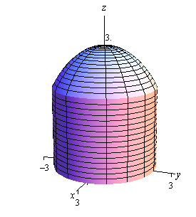
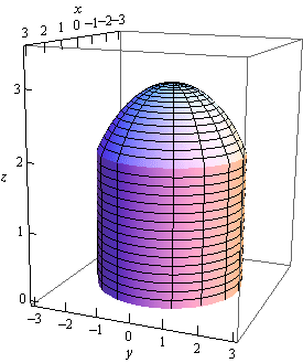
So, the region that we want the volume for is really a cylinder with a cap that comes from the sphere.
We are definitely going to want to do this integral in terms of polar coordinates so here are the limits (in polar coordinates) for the region,
\[\begin{array}{c}0 \le \theta \le 2\pi \\ 0 \le r \le \sqrt 5 \end{array}\]and we’ll need to convert the function to polar coordinates as well.
\[z = \sqrt {9 - \left( {{x^2} + {y^2}} \right)} = \sqrt {9 - {r^2}} \]The volume is then,
\[\begin{align*}V & = \iint\limits_{D}{{\sqrt {9 - {x^2} - {y^2}} \,dA}}\\ & = \int_{{\,0}}^{{\,2\pi }}{{\int_{{\,0}}^{{\,\sqrt 5 }}{{r\sqrt {9 - {r^2}} \,dr}}\,d\theta }}\\ & = \int_{{\,0}}^{{\,2\pi }}{{ - \frac{1}{3}\left. {{{\left( {9 - {r^2}} \right)}^{\frac{3}{2}}}} \right|_0^{\sqrt 5 }\,d\theta }}\\ & = \int_{{\,0}}^{{\,2\pi }}{{\frac{{19}}{3}\,d\theta }}\\ & = \frac{{38\pi }}{3}\end{align*}\]Let’s start this example off with a quick sketch of the region.
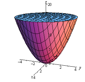
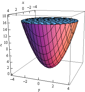
Now, in this case the standard formula is not going to work. The formula
\[V = \iint\limits_{D}{{f\left( {x,y} \right)\,dA}}\]finds the volume under the function \(f\left( {x,y} \right)\) and we’re actually after the volume that is above a function. This isn’t the problem that it might appear to be however. First, notice that
\[V = \iint\limits_{D}{{16\,dA}}\]will be the volume under \(z = 16\) (of course we’ll need to determine \(D\) eventually) while
\[V = \iint\limits_{D}{{{x^2} + {y^2}\,dA}}\]is the volume under \(z = {x^2} + {y^2}\), using the same \(D\).
The volume that we’re after is really the difference between these two or,
\[V = \iint\limits_{D}{{16\,dA}} - \iint\limits_{D}{{{x^2} + {y^2}\,dA}} = \iint\limits_{D}{{16 - \left( {{x^2} + {y^2}} \right)\,dA}}\]Now all that we need to do is to determine the region \(D\) and then convert everything over to polar coordinates.
Determining the region \(D\) in this case is not too bad. If we were to look straight down the \(z\)-axis onto the region we would see a circle of radius 4 centered at the origin. This is because the top of the region, where the elliptic paraboloid intersects the plane, is the widest part of the region. We know the \(z\) coordinate at the intersection so, setting \(z = 16\) in the equation of the paraboloid gives,
\[16 = {x^2} + {y^2}\]which is the equation of a circle of radius 4 centered at the origin.
Here are the inequalities for the region and the function we’ll be integrating in terms of polar coordinates.
\[0 \le \theta \le 2\pi \hspace{0.5in}0 \le r \le 4\hspace{0.5in}z = 16 - {r^2}\]The volume is then,
\[\begin{align*}V & = \iint\limits_{D}{{16 - \left( {{x^2} + {y^2}} \right)\,dA}}\\ & = \int_{{\,0}}^{{\,2\pi }}{{\int_{{\,0}}^{{\,4}}{{r\left( {16 - {r^2}} \right)\,dr}}\,d\theta }}\\ & = \int_{{\,0}}^{{\,2\pi }}{{\left. {\left( {8{r^2} - \frac{1}{4}{r^4}} \right)} \right|}}_0^4\,d\theta \\ & = \int_{{\,0}}^{{\,2\pi }}{{64\,d\theta }}\,\\ & = 128\pi \end{align*}\]In both of the previous volume problems we would have not been able to easily compute the volume without first converting to polar coordinates so, as these examples show, it is a good idea to always remember polar coordinates.
There is one more type of example that we need to look at before moving on to the next section. Sometimes we are given an iterated integral that is already in terms of \(x\) and \(y\) and we need to convert this over to polar so that we can actually do the integral. We need to see an example of how to do this kind of conversion.
First, notice that we cannot do this integral in Cartesian coordinates and so converting to polar coordinates may be the only option we have for actually doing the integral. Notice that the function will convert to polar coordinates nicely and so shouldn’t be a problem.
Let’s first determine the region that we’re integrating over and see if it’s a region that can be easily converted into polar coordinates. Here are the inequalities that define the region in terms of Cartesian coordinates.
\[\begin{array}{c} - 1 \le x \le 1\\ - \sqrt {1 - {x^2}} \le y \le 0\end{array}\]Now, the lower limit for the \(y\)’s is,
\[y = - \sqrt {1 - {x^2}} \]and this looks like the bottom of the circle of radius 1 centered at the origin. Since the upper limit for the \(y\)’s is \(y = 0\) we won’t have any portion of the top half of the disk and so it looks like we are going to have a portion (or all) of the bottom of the disk of radius 1 centered at the origin.
The range for the \(x\)’s in turn, tells us that we are will in fact have the complete bottom part of the disk.
So, we know that the inequalities that will define this region in terms of polar coordinates are then,
\[\begin{array}{c}\pi \le \theta \le 2\pi \\ 0 \le r \le 1\end{array}\]Finally, we just need to remember that,
\[dx\,dy = dA = r\,dr\,d\theta \]and so the integral becomes,
\[\int_{{ - 1}}^{1}{{\int_{{ - \sqrt {1 - {x^2}} }}^{0}{{\cos \left( {{x^2} + {y^2}} \right)\,dy}}\,dx}} = \int_{\pi }^{{2\pi }}{{\int_{0}^{1}{{r\cos \left( {{r^2}} \right)\,dr}}\,d\theta }}\]Note that this is an integral that we can do. So, here is the rest of the work for this integral.
\[\begin{align*}\int_{{ - 1}}^{1}{{\int_{{ - \sqrt {1 - {x^2}} }}^{0}{{\cos \left( {{x^2} + {y^2}} \right)\,dy}}\,dx}} & = \int_{\pi }^{{2\pi }}{{\left. {\frac{1}{2}\sin \left( {{r^2}} \right)} \right|_0^1\,d\theta }}\\ & = \int_{\pi }^{{2\pi }}{{\frac{1}{2}\sin \left( 1 \right)\,d\theta }}\\ & = \frac{\pi }{2}\sin \left( 1 \right)\end{align*}\]