Section 10.17 : Applications of Series
Now, that we know how to represent function as power series we can now talk about at least a couple of applications of series.
There are in fact many applications of series, unfortunately most of them are beyond the scope of this course. One application of power series (with the occasional use of Taylor Series) is in the field of Ordinary Differential Equations when finding Series Solutions to Differential Equations. If you are interested in seeing how that works you can check out that chapter of my Differential Equations notes.
Another application of series arises in the study of Partial Differential Equations. One of the more commonly used methods in that subject makes use of Fourier Series.
Many of the applications of series, especially those in the differential equations fields, rely on the fact that functions can be represented as a series. In these applications it is very difficult, if not impossible, to find the function itself. However, there are methods of determining the series representation for the unknown function.
While the differential equations applications are beyond the scope of this course there are some applications from a Calculus setting that we can look at.
To do this we will first need to find a Taylor Series about\(x = 0\) for the integrand. This however isn’t terribly difficult. We already have a Taylor Series for sine about \(x = 0\) so we’ll just use that as follows,
\[\frac{{\sin x}}{x} = \frac{1}{x}\sum\limits_{n = 0}^\infty {\frac{{{{\left( { - 1} \right)}^n}{x^{2n + 1}}}}{{\left( {2n + 1} \right)!}}} = \sum\limits_{n = 0}^\infty {\frac{{{{\left( { - 1} \right)}^n}{x^{2n}}}}{{\left( {2n + 1} \right)!}}} \]We can now do the problem.
\[\begin{align*}\int{{\frac{{\sin x}}{x}\,dx}} & = \int{{\sum\limits_{n = 0}^\infty {\frac{{{{\left( { - 1} \right)}^n}{x^{2n}}}}{{\left( {2n + 1} \right)!}}} \,dx}}\\ & = C + \sum\limits_{n = 0}^\infty {\frac{{{{\left( { - 1} \right)}^n}{x^{2n + 1}}}}{{\left( {2n + 1} \right)\,\,\left( {2n + 1} \right)!}}} \end{align*}\]So, while we can’t integrate this function in terms of known functions we can come up with a series representation for the integral.
This idea of deriving a series representation for a function instead of trying to find the function itself is used quite often in several fields. In fact, there are some fields where this is one of the main ideas used and without this idea it would be very difficult to accomplish anything in those fields.
Another application of series isn’t really an application of infinite series. It’s more an application of partial sums. In fact, we’ve already seen this application in use once in this chapter. In the Estimating the Value of a Series we used a partial sum to estimate the value of a series. We can do the same thing with power series and series representations of functions. The main difference is that we will now be using the partial sum to approximate a function instead of a single value.
We will look at Taylor series for our examples, but we could just as easily use any series representation here. Recall that the nth degree Taylor Polynomial of \(f\left( x \right)\) is given by,
\[{T_n}\left( x \right) = \sum\limits_{i = 0}^n {\frac{{{f^{\left( i \right)}}\left( a \right)}}{{i!}}{{\left( {x - a} \right)}^i}} \]Let’s take a look at example of this.
Here is the general formula for the Taylor polynomials for cosine.
\[{T_{2n}}\left( x \right) = \sum\limits_{i = 0}^n {\frac{{{{\left( { - 1} \right)}^i}{x^{2i}}}}{{\left( {2i} \right)!}}} \]The three Taylor polynomials that we’ve got are then,
\[\begin{align*}{T_2}\left( x \right) & = 1 - \frac{{{x^2}}}{2}\\ {T_4}\left( x \right) & = 1 - \frac{{{x^2}}}{2} + \frac{{{x^4}}}{{24}}\\ {T_8}\left( x \right) & = 1 - \frac{{{x^2}}}{2} + \frac{{{x^4}}}{{24}} - \frac{{{x^6}}}{{720}} + \frac{{{x^8}}}{{40320}}\end{align*}\]Here is the graph of these three Taylor polynomials as well as the graph of cosine.
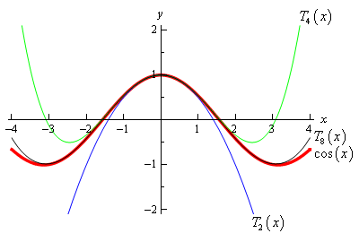
As we can see from this graph as we increase the degree of the Taylor polynomial it starts to look more and more like the function itself. In fact, by the time we get to \({T_8}\left( x \right)\) the only difference is right at the ends. The higher the degree of the Taylor polynomial the better it approximates the function.
Also, the larger the interval the higher degree Taylor polynomial we need to get a good approximation for the whole interval.
Before moving on let’s write down a couple more Taylor polynomials from the previous example. Notice that because the Taylor series for cosine doesn’t contain any terms with odd powers on \(x\) we get the following Taylor polynomials.
\[\begin{align*}{T_3}\left( x \right) & = 1 - \frac{{{x^2}}}{2}\\ {T_5}\left( x \right) & = 1 - \frac{{{x^2}}}{2} + \frac{{{x^4}}}{{24}}\\ {T_9}\left( x \right) & = 1 - \frac{{{x^2}}}{2} + \frac{{{x^4}}}{{24}} - \frac{{{x^6}}}{{720}} + \frac{{{x^8}}}{{40320}}\end{align*}\]These are identical to those used in the example. Sometimes this will happen although that was not really the point of this. The point is to notice that the nth degree Taylor polynomial may actually have a degree that is less than \(n\). It will never be more than \(n\), but it can be less than \(n\).
The final example in this section really isn’t an application of series and probably belonged in the previous section. However, the previous section was getting too long so the example is in this section. This is an example of how to multiply series together and while this isn’t an application of series it is something that does have to be done on occasion in the applications. So, in that sense it does belong in this section.
Before we start let’s acknowledge that the easiest way to do this problem is to simply compute the first 3-4 derivatives, evaluate them at \(x = 0\), plug into the formula and we’d be done. However, as we noted prior to this example we want to use this example to illustrate how we multiply series.
We will make use of the fact that we’ve got Taylor Series for each of these so we can use them in this problem.
\[{{\bf{e}}^x}\cos x = \left( {\sum\limits_{n = 0}^\infty {\frac{{{x^n}}}{{n!}}} } \right)\left( {\sum\limits_{n = 0}^\infty {\frac{{{{\left( { - 1} \right)}^n}{x^{2n}}}}{{\left( {2n} \right)!}}} } \right)\]We’re not going to completely multiply out these series. We’re going to do enough of the multiplication to get an answer. The problem statement says that we want the first three non-zero terms. That non-zero bit is important as it is possible that some of the terms will be zero. If none of the terms are zero this would mean that the first three non-zero terms would be the constant term, \(x\) term, and \({x^2}\) term. However, because some might be zero let’s assume that if we get all the terms up through \({x^4}\) we’ll have enough to get the answer. If we’ve assumed wrong it will be very easy to fix so don’t worry about that.
Now, let’s write down the first few terms of each series and we’ll stop at the x4 term in each.
\[{{\bf{e}}^x}\cos x = \left( {1 + x + \frac{{{x^2}}}{2} + \frac{{{x^3}}}{6} + \frac{{{x^4}}}{{24}} + \cdots } \right)\left( {1 - \frac{{{x^2}}}{2} + \frac{{{x^4}}}{{24}} + \cdots } \right)\]Note that we do need to acknowledge that these series don’t stop. That’s the purpose of the “\( + \cdots \)” at the end of each. Just for a second however, let’s suppose that each of these did stop and ask ourselves how we would multiply each out. If this were the case we would take every term in the second and multiply by every term in the first. In other words, we would first multiply every term in the second series by 1, then every term in the second series by \(x\), then by \({x^2}\) etc.
By stopping each series at \({x^4}\) we have now guaranteed that we’ll get all terms that have an exponent of 4 or less. Do you see why?
Each of the terms that we neglected to write down have an exponent of at least 5 and so multiplying by 1 or any power of \(x\) will result in a term with an exponent that is at a minimum 5. Therefore, none of the neglected terms will contribute terms with an exponent of 4 or less and so weren’t needed.
So, let’s start the multiplication process.
\[\begin{align*}{{\bf{e}}^x}\cos x & = \left( {1 + x + \frac{{{x^2}}}{2} + \frac{{{x^3}}}{6} + \frac{{{x^4}}}{{24}} + \cdots } \right)\left( {1 - \frac{{{x^2}}}{2} + \frac{{{x^4}}}{{24}} + \cdots } \right)\\ & = \underbrace {1 - \frac{{{x^2}}}{2} + \frac{{{x^4}}}{{24}} + \cdots }_{{\mbox{Second Series }} \times {\mbox{ 1}}} + \underbrace {x - \frac{{{x^3}}}{2} + \frac{{{x^5}}}{{24}} + \cdots }_{{\mbox{Second Series }} \times {\mbox{ }}x} + \underbrace {\frac{{{x^2}}}{2} - \frac{{{x^4}}}{4} + \frac{{{x^6}}}{{48}} + \cdots }_{{\mbox{Second Series }} \times {\mbox{ }}{\displaystyle{}^{{{x^2}}}/{}_{2}}}\\ & \hspace{0.75in} + \underbrace {\frac{{{x^3}}}{6} - \frac{{{x^5}}}{{12}} + \frac{{{x^7}}}{{144}} + \cdots }_{{\mbox{Second Series }} \times {\mbox{ }}{\displaystyle{}^{{{x^3}}}/{}_{6}}} + \underbrace {\frac{{{x^4}}}{{24}} - \frac{{{x^6}}}{{48}} + \frac{{{x^8}}}{{576}} + \cdots }_{{\mbox{Second Series }} \times {\mbox{ }}{\displaystyle{}^{{{x^4}}}/{}_{{24}}}} + \cdots \end{align*}\]Now, collect like terms ignoring everything with an exponent of 5 or more since we won’t have all those terms and don’t want them either. Doing this gives,
\[\begin{align*}{{\bf{e}}^x}\cos x & = 1 + x + \left( { - \frac{1}{2} + \frac{1}{2}} \right){x^2} + \left( { - \frac{1}{2} + \frac{1}{6}} \right){x^3} + \left( {\frac{1}{{24}} - \frac{1}{4} + \frac{1}{{24}}} \right){x^4} + \cdots \\ & = 1 + x - \frac{{{x^3}}}{3} - \frac{{{x^4}}}{6} + \cdots \end{align*}\]There we go. It looks like we over guessed and ended up with four non-zero terms, but that’s okay. If we had under guessed and it turned out that we needed terms with \({x^5}\) in them all we would need to do at this point is go back and add in those terms to the original series and do a couple quick multiplications. In other words, there is no reason to completely redo all the work.