Section 2.7 : Modeling with First Order Differential Equations
We now move into one of the main applications of differential equations both in this class and in general. Modeling is the process of writing a differential equation to describe a physical situation. Almost all of the differential equations that you will use in your job (for the engineers out there in the audience) are there because somebody, at some time, modeled a situation to come up with the differential equation that you are using.
This section is not intended to completely teach you how to go about modeling all physical situations. A whole course could be devoted to the subject of modeling and still not cover everything! This section is designed to introduce you to the process of modeling and show you what is involved in modeling. We will look at three different situations in this section : Mixing Problems, Population Problems, and Falling Objects.
In all of these situations we will be forced to make assumptions that do not accurately depict reality in most cases, but without them the problems would be very difficult and beyond the scope of this discussion (and the course in most cases to be honest).
So, let’s get started.
Mixing Problems
In these problems we will start with a substance that is dissolved in a liquid. Liquid will be entering and leaving a holding tank. The liquid entering the tank may or may not contain more of the substance dissolved in it. Liquid leaving the tank will of course contain the substance dissolved in it. If \(Q(t)\) gives the amount of the substance dissolved in the liquid in the tank at any time \(t\) we want to develop a differential equation that, when solved, will give us an expression for \(Q(t)\). Note as well that in many situations we can think of air as a liquid for the purposes of these kinds of discussions and so we don’t actually need to have an actual liquid but could instead use air as the “liquid”.
The main assumption that we’ll be using here is that the concentration of the substance in the liquid is uniform throughout the tank. Clearly this will not be the case, but if we allow the concentration to vary depending on the location in the tank the problem becomes very difficult and will involve partial differential equations, which is not the focus of this course.
The main “equation” that we’ll be using to model this situation is :
| Rate of change of \(Q(t)\) |
= | Rate at which \(Q(t)\) enters the tank |
– | Rate at which \(Q(t)\) exits the tank |
where,
| Rate of change of \(Q(t)\) : \(\displaystyle \frac{{dQ}}{{dt}} = Q'\left( t \right)\) |
| Rate at which \(Q(t)\) enters the tank : (flow rate of liquid entering) x (concentration of substance in liquid entering) |
| Rate at which \(Q(t)\) exits the tank : (flow rate of liquid exiting) x (concentration of substance in liquid exiting) |
Let’s take a look at the first problem.
First off, let’s address the “well mixed solution” bit. This is the assumption that was mentioned earlier. We are going to assume that the instant the water enters the tank it somehow instantly disperses evenly throughout the tank to give a uniform concentration of salt in the tank at every point. Again, this will clearly not be the case in reality, but it will allow us to do the problem.
Now, to set up the IVP that we’ll need to solve to get \(Q(t)\) we’ll need the flow rate of the water entering (we’ve got that), the concentration of the salt in the water entering (we’ve got that), the flow rate of the water leaving (we’ve got that) and the concentration of the salt in the water exiting (we don’t have this yet).
So, we first need to determine the concentration of the salt in the water exiting the tank. Since we are assuming a uniform concentration of salt in the tank the concentration at any point in the tank and hence in the water exiting is given by,
\[{\mbox{Concentration}} = \frac{{{\mbox{Amount of salt in the tank at any time, }}t}}{{{\mbox{Volume of water in the tank at any time, }}t}}\]The amount at any time \(t\) is easy it’s just \(Q(t)\). The volume is also pretty easy. We start with 600 gallons and every hour 9 gallons enters and 6 gallons leave. So, if we use \(t\) in hours, every hour 3 gallons enters the tank, or at any time \(t\) there is 600 + 3\(t\) gallons of water in the tank.
So, the IVP for this situation is,
\[\begin{align*}Q'\left( t \right) & = \left( 9 \right)\left( {\frac{1}{5}\left( {1 + \cos \left( t \right)} \right)} \right) - \left( 6 \right)\left( {\frac{{Q\left( t \right)}}{{600 + 3t}}} \right)\hspace{0.25in}Q\left( 0 \right) = 5\\ Q'\left( t \right) & = \frac{9}{5}\left( {1 + \cos \left( t \right)} \right) - \frac{{2Q\left( t \right)}}{{200 + t}}\hspace{0.25in}Q\left( 0 \right) = 5\end{align*}\]This is a linear differential equation and it isn’t too difficult to solve (hopefully). We will show most of the details but leave the description of the solution process out. If you need a refresher on solving linear first order differential equations go back and take a look at that section.
\[Q'\left( t \right) + \frac{{2Q\left( t \right)}}{{200 + t}} = \frac{9}{5}\left( {1 + \cos \left( t \right)} \right)\] \[\mu \left( t \right) = {{\bf{e}}^{\int{{\frac{2}{{200 + t}}dt}}}} = {{\bf{e}}^{2\ln \left( {200 + t} \right)}} = {\left( {200 + t} \right)^2}\] \[\int{{{{\left( {{{\left( {200 + t} \right)}^2}Q\left( t \right)} \right)}^\prime }\,dt}}\, = \int{{\frac{9}{5}{{\left( {200 + t} \right)}^2}\left( {1 + \cos \left( t \right)} \right)dt}}\] \[\begin{align*}{\left( {200 + t} \right)^2}Q\left( t \right) & = \frac{9}{5}\left( {\frac{1}{3}{{\left( {200 + t} \right)}^3} + {{\left( {200 + t} \right)}^2}\sin \left( t \right) + 2\left( {200 + t} \right)\cos \left( t \right) - 2\sin \left( t \right)} \right) + c\\ Q\left( t \right) & = \frac{9}{5}\left( {\frac{1}{3}\left( {200 + t} \right) + \sin \left( t \right) + \frac{{2\cos \left( t \right)}}{{200 + t}} - \frac{{2\sin \left( t \right)}}{{{{\left( {200 + t} \right)}^2}}}} \right) + \frac{c}{{{{\left( {200 + t} \right)}^2}}}\end{align*}\]So, here’s the general solution. Now, apply the initial condition to get the value of the constant, \(c\).
\[5 = Q\left( 0 \right) = \frac{9}{5}\left( {\frac{1}{3}\left( {200} \right) + \frac{2}{{200}}} \right) + \frac{c}{{{{\left( {200} \right)}^2}}}\hspace{0.25in}c = - 4600720\]So, the amount of salt in the tank at any time \(t\) is.
\[Q\left( t \right) = \frac{9}{5}\left( {\frac{1}{3}\left( {200 + t} \right) + \sin \left( t \right) + \frac{{2\cos \left( t \right)}}{{200 + t}} - \frac{{2\sin \left( t \right)}}{{{{\left( {200 + t} \right)}^2}}}} \right) - \frac{{4600720}}{{{{\left( {200 + t} \right)}^2}}}\]Now, the tank will overflow at \(t\) = 300 hrs. The amount of salt in the tank at that time is.
\[Q\left( {300} \right) = 279.797{\mbox{ lbs}}\]Here’s a graph of the salt in the tank before it overflows.
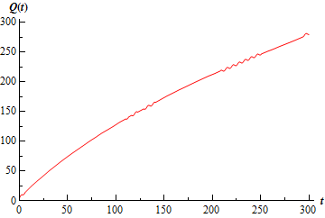
Note that the whole graph should have small oscillations in it as you can see in the range from 200 to 250. The scale of the oscillations however was small enough that the program used to generate the image had trouble showing all of them.
The work was a little messy with that one, but they will often be that way so don’t get excited about it. This first example also assumed that nothing would change throughout the life of the process. That, of course, will usually not be the case. Let’s take a look at an example where something changes in the process.
Okay, so clearly the pollution in the tank will increase as time passes. If the amount of pollution ever reaches the maximum allowed there will be a change in the situation. This will necessitate a change in the differential equation describing the process as well. In other words, we’ll need two IVP’s for this problem. One will describe the initial situation when polluted runoff is entering the tank and one for after the maximum allowed pollution is reached and fresh water is entering the tank.
Here are the two IVP’s for this problem.
\[\begin{align*}{Q_1}^\prime \left( t \right) & = \left( 3 \right)\left( 5 \right) - \left( 3 \right)\left( {\frac{{{Q_1}\left( t \right)}}{{800}}} \right)\hspace{0.25in}{Q_1}\left( 0 \right) = 2\hspace{0.25in}0 \le t \le {t_m}\\ {Q_2}^\prime \left( t \right) & = \left( 2 \right)\left( 0 \right) - \left( 4 \right)\left( {\frac{{{Q_2}\left( t \right)}}{{800 - 2\left( {t - {t_m}} \right)}}} \right)\hspace{0.25in}{Q_2}\left( {{t_m}} \right) = 500\hspace{0.25in}{t_m} \le t \le {t_e}\end{align*}\]The first one is fairly straight forward and will be valid until the maximum amount of pollution is reached. We’ll call that time \(t_{m}\). Also, the volume in the tank remains constant during this time so we don’t need to do anything fancy with that this time in the second term as we did in the previous example.
We’ll need a little explanation for the second one. First notice that we don’t “start over” at \(t = 0\). We start this one at \(t_{m}\), the time at which the new process starts. Next, fresh water is flowing into the tank and so the concentration of pollution in the incoming water is zero. This will drop out the first term, and that’s okay so don’t worry about that.
Now, notice that the volume at any time looks a little funny. During this time frame we are losing two gallons of water every hour of the process so we need the “-2” in there to account for that. However, we can’t just use \(t\) as we did in the previous example. When this new process starts up there needs to be 800 gallons of water in the tank and if we just use \(t\) there we won’t have the required 800 gallons that we need in the equation. So, to make sure that we have the proper volume we need to put in the difference in times. In this way once we are one hour into the new process (i.e \(t - t_{m} = 1\)) we will have 798 gallons in the tank as required.
Finally, the second process can’t continue forever as eventually the tank will empty. This is denoted in the time restrictions as \(t_{e}\). We can also note that \(t_{e} = t_{m} + 400\) since the tank will empty 400 hours after this new process starts up. Well, it will end provided something doesn’t come along and start changing the situation again.
Okay, now that we’ve got all the explanations taken care of here’s the simplified version of the IVP’s that we’ll be solving.
\[\begin{align*}{Q_1}^\prime \left( t \right) & = 15 - \frac{{3{Q_1}\left( t \right)}}{{800}}\hspace{0.25in}{Q_1}\left( 0 \right) = 2\hspace{0.25in}0 \le t \le {t_m}\\ {Q_2}^\prime \left( t \right) & = - \frac{{2{Q_2}\left( t \right)}}{{400 - \left( {t - {t_m}} \right)}}\hspace{0.25in}{Q_2}\left( {{t_m}} \right) = 500\hspace{0.25in}{t_m} \le t \le {t_e}\end{align*}\]The first IVP is a fairly simple linear differential equation so we’ll leave the details of the solution to you to check. Upon solving you get.
\[{Q_1}\left( t \right) = 4000 - 3998{{\bf{e}}^{ - \,\,\frac{{3\,t}}{{800}}}}\]Now, we need to find \(t_{m}\). This isn’t too bad all we need to do is determine when the amount of pollution reaches 500. So, we need to solve.
\[{Q_1}\left( t \right) = 4000 - 3998{{\bf{e}}^{ - \,\,\frac{{3\,t}}{{800}}}} = 500\hspace{0.25in} \Rightarrow \hspace{0.25in}{t_m} = 35.4750\]So, the second process will pick up at 35.475 hours. For completeness sake here is the IVP with this information inserted.
\[{Q_2}^\prime \left( t \right) = - \frac{{2{Q_2}\left( t \right)}}{{435.475 - t}}\hspace{0.25in}{Q_2}\left( {35.475} \right) = 500\hspace{0.25in}35.475 \le t \le 435.475\]This differential equation is both linear and separable and again isn’t terribly difficult to solve so I’ll leave the details to you again to check that we should get.
\[{Q_2}\left( t \right) = \frac{{{{\left( {435.476 - t} \right)}^2}}}{{320}}\]So, a solution that encompasses the complete running time of the process is
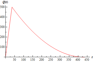
\[Q\left( t \right) = \left\{ {\begin{array}{*{20}{l}}{4000 - 3998{{\bf{e}}^{ - \,\,\frac{{3\,t}}{{800}}}}}&{\hspace{0.25in}0 \le t \le 35.475}\\{\displaystyle \frac{{{{\left( {435.476 - t} \right)}^2}}}{{320}}}&{\hspace{0.25in}35.475 \le t \le 435.4758}\end{array}} \right.\]Here is a graph of the amount of pollution in the tank at any time \(t\).
As you can surely see, these problems can get quite complicated if you want them to. Take the last example. A more realistic situation would be that once the pollution dropped below some predetermined point the polluted runoff would, in all likelihood, be allowed to flow back in and then the whole process would repeat itself. So, realistically, there should be at least one more IVP in the process.
Let’s move on to another type of problem now.
Population
These are somewhat easier than the mixing problems although, in some ways, they are very similar to mixing problems. So, if \(P(t)\) represents a population in a given region at any time \(t\) the basic equation that we’ll use is identical to the one that we used for mixing. Namely,
| Rate of change of \(P(t)\) |
= | Rate at which \(P(t)\) enters the region |
- | Rate at which \(P(t)\) exits the region |
Here the rate of change of \(P(t)\) is still the derivative. What’s different this time is the rate at which the population enters and exits the region. For population problems all the ways for a population to enter the region are included in the entering rate. Birth rate and migration into the region are examples of terms that would go into the rate at which the population enters the region. Likewise, all the ways for a population to leave an area will be included in the exiting rate. Therefore, things like death rate, migration out and predation are examples of terms that would go into the rate at which the population exits the area.
Here’s an example.
Let’s start out by looking at the birth rate. We are told that the insects will be born at a rate that is proportional to the current population. This means that the birth rate can be written as
\[rP\]where \(r\) is a positive constant that will need to be determined. Now, let’s take everything into account and get the IVP for this problem.
\[\begin{align*}P' & = \left( {rP + 15} \right) - \left( {16 + 7} \right)\hspace{0.25in}P\left( 0 \right) = 100\\ P' & = rP - 8\hspace{0.25in}P\left( 0 \right) = 100\end{align*}\]Note that in the first line we used parenthesis to note which terms went into which part of the differential equation. Also note that we don’t make use of the fact that the population will triple in two weeks time in the absence of outside factors here. In the absence of outside factors means that the ONLY thing that we can consider is birth rate. Nothing else can enter into the picture and clearly we have other influences in the differential equation.
So, just how does this tripling come into play? Well, we should also note that without knowing \(r\) we will have a difficult time solving the IVP completely. We will use the fact that the population triples in two weeks time to help us find \(r\). In the absence of outside factors the differential equation would become.
\[P' = rP\hspace{0.25in}P\left( 0 \right) = 100\hspace{0.25in}P\left( {14} \right) = 300\]Note that since we used days as the time frame in the actual IVP I needed to convert the two weeks to 14 days. We could have just as easily converted the original IVP to weeks as the time frame, in which case there would have been a net change of –56 per week instead of the –8 per day that we are currently using in the original differential equation.
Okay back to the differential equation that ignores all the outside factors. This differential equation is separable and linear (either can be used) and is a simple differential equation to solve. We’ll leave the detail to you to get the general solution.
\[P\left( t \right) = c{{\bf{e}}^{rt}}\]Applying the initial condition gives \(c\) = 100. Now apply the second condition.
\[300 = P\left( {14} \right) = 100{{\bf{e}}^{14r}}\hspace{0.25in}300 = 100{{\bf{e}}^{14r}}\]We need to solve this for \(r\). First divide both sides by 100, then take the natural log of both sides.
\[\begin{align*}3 & = {{\bf{e}}^{14r}}\\ \ln 3 & = \ln {{\bf{e}}^{14r}}\\ \ln 3 & = 14r\\ r & = \frac{{\ln 3}}{{14}}\end{align*}\]We made use of the fact that \(\ln {{\bf{e}}^{g\left( x \right)}} = g\left( x \right)\) here to simplify the problem. Now, that we have \(r\) we can go back and solve the original differential equation. We’ll rewrite it a little for the solution process.
\[P' - \frac{{\ln 3}}{{14}}P = - 8\hspace{0.25in}P\left( 0 \right) = 100\]This is a fairly simple linear differential equation, but that coefficient of \(P\) always get people bent out of shape, so we’ll go through at least some of the details here.
\[\mu \left( t \right) = {{\bf{e}}^{\int{{ - \,\frac{{\ln 3}}{{14}}dt}}}} = {{\bf{e}}^{ - \,\,\frac{{\ln 3}}{{14}}\,t}}\]Now, don’t get excited about the integrating factor here. It’s just like \({{\bf{e}}^{2t}}\) only this time the constant is a little more complicated than just a 2, but it is a constant! Now, solve the differential equation.
\[\begin{align*}\int{{{{\left( {P{{\bf{e}}^{ - \,\,\frac{{\ln 3}}{{14}}\,t}}} \right)}^\prime }\,dt}} & = \int{{ - 8{{\bf{e}}^{ - \,\,\frac{{\ln 3}}{{14}}\,t}}\,dt}}\\ P{{\bf{e}}^{ - \,\,\frac{{\ln 3}}{{14}}\,t}} & = - 8\left( { - \frac{{14}}{{\ln 3}}} \right){{\bf{e}}^{ - \,\,\frac{{\ln 3}}{{14}}\,t}} + c\\ P\left( t \right) & = \frac{{112}}{{\ln 3}} + c{{\bf{e}}^{\frac{{\ln 3}}{{14}}\,t}}\end{align*}\]Again, do not get excited about doing the right hand integral, it’s just like integrating \({{\bf{e}}^{2t}}\)! Applying the initial condition gives the following.
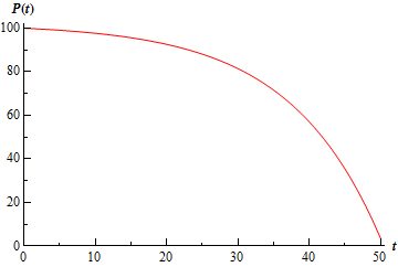
\[P\left( t \right) = \frac{{112}}{{\ln 3}} + \left( {100 - \frac{{112}}{{\ln 3}}} \right){{\bf{e}}^{\frac{{\ln 3}}{{14}}\,t}} = \frac{{112}}{{\ln 3}} - 1.94679{{\bf{e}}^{\frac{{\ln 3}}{{14}}\,t}}\]Now, the exponential has a positive exponent and so will go to plus infinity as \(t\) increases. Its coefficient, however, is negative and so the whole population will go negative eventually. Clearly, population can’t be negative, but in order for the population to go negative it must pass through zero. In other words, eventually all the insects must die. So, they don’t survive, and we can solve the following to determine when they die out.
\[0 = \frac{{112}}{{\ln 3}} - 1.94679{{\bf{e}}^{\frac{{\ln 3}}{{14}}\,t}}\hspace{0.25in} \Rightarrow \hspace{0.25in}t = 50.4415\,{\mbox{days}}\]So, the insects will survive for around 7.2 weeks. Here is a graph of the population during the time in which they survive.
As with the mixing problems, we could make the population problems more complicated by changing the circumstances at some point in time. For instance, if at some point in time the local bird population saw a decrease due to disease they wouldn’t eat as much after that point and a second differential equation to govern the time after this point.
Let’s now take a look at the final type of problem that we’ll be modeling in this section.
Falling Object
This will not be the first time that we’ve looked into falling bodies. If you recall, we looked at one of these when we were looking at Direction Fields. In that section we saw that the basic equation that we’ll use is Newton’s Second Law of Motion.
\[mv' = F\left( {t,v} \right)\]The two forces that we’ll be looking at here are gravity and air resistance. The main issue with these problems is to correctly define conventions and then remember to keep those conventions. By this we mean define which direction will be termed the positive direction and then make sure that all your forces match that convention. This is especially important for air resistance as this is usually dependent on the velocity and so the “sign” of the velocity can and does affect the “sign” of the air resistance force.
Let’s take a look at an example.
First, notice that when we say straight up, we really mean straight up, but in such a way that it will miss the bridge on the way back down. Here is a sketch of the situation.

Notice the conventions that we set up for this problem. Since the vast majority of the motion will be in the downward direction we decided to assume that everything acting in the downward direction should be positive. Note that we also defined the “zero position” as the bridge, which makes the ground have a “position” of 100.
Okay, if you think about it we actually have two situations here. The initial phase in which the mass is rising in the air and the second phase when the mass is on its way down. We will need to examine both situations and set up an IVP for each. We will do this simultaneously. Here are the forces that are acting on the object on the way up and on the way down.
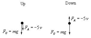
Notice that the air resistance force needs a negative in both cases in order to get the correct “sign” or direction on the force. When the mass is moving upwards the velocity (and hence \(v\)) is negative, yet the force must be acting in a downward direction. Therefore, the “-” must be part of the force to make sure that, overall, the force is positive and hence acting in the downward direction. Likewise, when the mass is moving downward the velocity (and so \(v\)) is positive. Therefore, the air resistance must also have a “-” in order to make sure that it’s negative and hence acting in the upward direction.
So, the IVP for each of these situations are.
\[\begin{array}{*{20}{c}}\begin{aligned}&\hspace{0.5in}{\mbox{Up}}\\ & mv' = mg - 5v\\ & v\left( 0 \right) = - 10\end{aligned}&\begin{aligned}&\hspace{0.35in}{\mbox{Down}}\\ & mv' = mg - 5v\\ & v\left( {{t_0}} \right) = 0\end{aligned}\end{array}\]In the second IVP, the \(t\)0 is the time when the object is at the highest point and is ready to start on the way down. Note that at this time the velocity would be zero. Also note that the initial condition of the first differential equation will have to be negative since the initial velocity is upward.
In this case, the differential equation for both of the situations is identical. This won’t always happen, but in those cases where it does, we can ignore the second IVP and just let the first govern the whole process.
So, let’s actually plug in for the mass and gravity (we’ll be using \(g\) = 9.8 m/s2 here). We’ll go ahead and divide out the mass while we’re at it since we’ll need to do that eventually anyway.
\[v' = 9.8 - \frac{{5v}}{{50}} = 9.8 - \frac{v}{{10}}\hspace{0.25in}v\left( 0 \right) = - 10\]This is a simple linear differential equation to solve so we’ll leave the details to you. Upon solving we arrive at the following equation for the velocity of the object at any time \(t\).
\[v\left( t \right) = 98 - 108{{\bf{e}}^{ - \,\frac{{t\,}}{{10}}}}\]Okay, we want the velocity of the ball when it hits the ground. Of course we need to know when it hits the ground before we can ask this. In order to find this we will need to find the position function. This is easy enough to do.
\[s\left( t \right) = \int{{v\left( t \right)\,dt}} = \int{{98 - 108{{\bf{e}}^{ - \,\frac{{t\,}}{{10}}}}\,dt}} = 98t + 1080{{\bf{e}}^{ - \,\frac{{t\,}}{{10}}}} + c\]We can now use the fact that I took the convention that \(s\)(0) = 0 to find that \(c\) = -1080. The position at any time is then.
\[s\left( t \right) = 98t + 1080{{\bf{e}}^{ - \,\frac{{t\,}}{{10}}}} - 1080\]To determine when the mass hits the ground we just need to solve.
\[100 = 98t + 1080{{\bf{e}}^{ - \,\frac{{t\,}}{{10}}}} - 1080\hspace{0.25in}t = - 3.32203,\,\,5.98147\]We’ve got two solutions here, but since we are starting things at \(t\) = 0, the negative is clearly the incorrect value. Therefore, the mass hits the ground at \(t\) = 5.98147. The velocity of the object upon hitting the ground is then.
\[v\left( {5.98147} \right) = 38.61841\]This last example gave us an example of a situation where the two differential equations needed for the problem ended up being identical and so we didn’t need the second one after all. Be careful however to not always expect this. We could very easily change this problem so that it required two different differential equations. For instance we could have had a parachute on the mass open at the top of its arc changing its air resistance. This would have completely changed the second differential equation and forced us to use it as well. Or, we could have put a river under the bridge so that before it actually hit the ground it would have first had to go through some water which would have a different “air” resistance for that phase necessitating a new differential equation for that portion.
Or, we could be really crazy and have both the parachute and the river which would then require three IVP’s to be solved before we determined the velocity of the mass before it actually hits the solid ground.
Finally, we could use a completely different type of air resistance that requires us to use a different differential equation for both the upwards and downwards portion of the motion. Let’s take a quick look at an example of this.
So, this is basically the same situation as in the previous example. We just changed the air resistance from \(5v\) to \(5{v^2}\). Also, we are just going to find the velocity at any time \(t\) for this problem because, we’ll see that the solution is really unpleasant and finding the velocity for when the mass hits the ground is simply more work than we want to put into a problem designed to illustrate the fact that we need a separate differential equation for both the upwards and downwards motion of the mass.
As with the previous example we will use the convention that everything downwards is positive. Here are the forces on the mass when the object is on the way up and on the way down.

Now, in this case, when the object is moving upwards the velocity is negative. However, because of the \({v^2}\) in the air resistance we do not need to add in a minus sign this time to make sure the air resistance is positive as it should be given that it is a downwards acting force.
On the downwards phase, however, we still need the minus sign on the air resistance given that it is an upwards force and so should be negative but the \({v^2}\) is positive.
This leads to the following IVP’s for each case.
\[\begin{array}{*{20}{c}}\begin{aligned}&\hspace{0.5in}{\mbox{Up}}\\ & mv' = mg + 5{v^2}\\ & v' = 9.8 + \frac{1}{{10}}{v^2}\\ & v\left( 0 \right) = - 10\end{aligned}&\begin{aligned}&\hspace{0.35in}{\mbox{Down}}\\ & mv' = mg - 5{v^2}\\ & v' = 9.8 - \frac{1}{{10}}{v^2}\\ & v\left( {{t_0}} \right) = 0\end{aligned}\end{array}\]
These are clearly different differential equations and so, unlike the previous example, we can’t just use the first for the full problem.
Also, the solution process for these will be a little more involved than the previous example as neither of the differential equations are linear. They are both separable differential equations however.
So, let’s get the solution process started. We will first solve the upwards motion differential equation. Here is the work for solving this differential equation.
\[\begin{align*}\int{{\frac{1}{{9.8 + \frac{1}{{10}}{v^2}}}\,dv}} & = \int{{dt}}\\ 10\int{{\frac{1}{{98 + {v^2}}}\,dv}} & = \int{{dt}}\\ \frac{{10}}{{\sqrt {98} }}{\tan ^{ - 1}}\left( {\frac{v}{{\sqrt {98} }}} \right) & = t + c\end{align*}\]Note that we did a little rewrite on the integrand to make the process a little easier in the second step.
Now, we have two choices on proceeding from here. Either we can solve for the velocity now, which we will need to do eventually, or we can apply the initial condition at this stage. While, we’ve always solved for the function before applying the initial condition we could just as easily apply it here if we wanted to and, in this case, will probably be a little easier.
So, to apply the initial condition all we need to do is recall that \(v\) is really \(v\left( t \right)\) and then plug in \(t = 0\). Doing this gives,
\[\frac{{10}}{{\sqrt {98} }}{\tan ^{ - 1}}\left( {\frac{{v\left( 0 \right)}}{{\sqrt {98} }}} \right) = 0 + c\]
Now, all we need to do is plug in the fact that we know \(v\left( 0 \right) = - 10\) to get.
\[c = \frac{{10}}{{\sqrt {98} }}{\tan ^{ - 1}}\left( {\frac{{ - 10}}{{\sqrt {98} }}} \right)\]
Messy, but there it is. The velocity for the upward motion of the mass is then,
\[\begin{align*}\frac{{10}}{{\sqrt {98} }}{\tan ^{ - 1}}\left( {\frac{v}{{\sqrt {98} }}} \right) & = t + \frac{{10}}{{\sqrt {98} }}{\tan ^{ - 1}}\left( {\frac{{ - 10}}{{\sqrt {98} }}} \right)\\ {\tan ^{ - 1}}\left( {\frac{v}{{\sqrt {98} }}} \right) & = \frac{{\sqrt {98} }}{{10}}t + {\tan ^{ - 1}}\left( {\frac{{ - 10}}{{\sqrt {98} }}} \right)\\ v\left( t \right) & = \sqrt {98} \tan \left( {\frac{{\sqrt {98} }}{{10}}t + {{\tan }^{ - 1}}\left( {\frac{{ - 10}}{{\sqrt {98} }}} \right)} \right)\end{align*}\]
Now, we need to determine when the object will reach the apex of its trajectory. To do this all we need to do is set this equal to zero given that the object at the apex will have zero velocity right before it starts the downward motion. We will leave it to you to verify that the velocity is zero at the following values of \(t\).
\[t = \frac{{10}}{{\sqrt {98} }}\left[ {{{\tan }^{ - 1}}\left( {\frac{{10}}{{\sqrt {98} }}} \right) + \pi n} \right]\hspace{0.25in}n = 0, \pm 1, \pm 2, \pm 3, \ldots \]
We clearly do not want all of these. We want the first positive \(t\) that will give zero velocity. It doesn’t make sense to take negative \(t\)’s given that we are starting the process at \(t = 0\) and once it hit’s the apex (i.e. the first positive \(t\) for which the velocity is zero) the solution is no longer valid as the object will start to move downwards and this solution is only for upwards motion.
Plugging in a few values of \(n\) will quickly show us that the first positive \(t\) will occur for \(n = 0\) and will be \(t = 0.79847\). We reduced the answer down to a decimal to make the rest of the problem a little easier to deal with.
The IVP for the downward motion of the object is then,
\[v' = 9.8 - \frac{1}{{10}}{v^2}\hspace{0.25in}v\left( {0.79847} \right) = 0\]
Now, this is also a separable differential equation, but it is a little more complicated to solve. First, let’s separate the differential equation (with a little rewrite) and at least put integrals on it.
\[\int{{\frac{1}{{9.8 - \frac{1}{{10}}{v^2}}}\,dv}} = 10\int{{\frac{1}{{98 - {v^2}}}\,dv}} = \int{{dt}}\]
The problem here is the minus sign in the denominator. Because of that this is not an inverse tangent as was the first integral. To evaluate this integral we could either do a trig substitution (\(v = \sqrt {98} \sin \theta \)) or use partial fractions using the fact that \(98 - {v^2} = \left( {\sqrt {98} - v} \right)\left( {\sqrt {98} + v} \right)\). You’re probably not used to factoring things like this but the partial fraction work allows us to avoid the trig substitution and it works exactly like it does when everything is an integer and so we’ll do that for this integral.
We’ll leave the details of the partial fractioning to you. Once the partial fractioning has been done the integral becomes,
\[\begin{align*}10\left( {\frac{1}{{2\sqrt {98} }}} \right)\int{{\frac{1}{{\sqrt {98} + v}} + \frac{1}{{\sqrt {98} - v}}\,dv}} & = \int{{dt}}\\ \frac{5}{{\sqrt {98} }}\left[ {\ln \left| {\sqrt {98} + v} \right| - \ln \left| {\sqrt {98} - v} \right|} \right] & = t + c\\ \frac{5}{{\sqrt {98} }}\ln \left| {\frac{{\sqrt {98} + v}}{{\sqrt {98} - v}}} \right| & = t + c\end{align*}\]
Again, we will apply the initial condition at this stage to make our life a little easier. Doing this gives,
\[\begin{align*}\frac{5}{{\sqrt {98} }}\ln \left| {\frac{{\sqrt {98} + v\left( {0.79847} \right)}}{{\sqrt {98} - v(0.79847}}} \right| & = 0.79847 + c\\ \frac{5}{{\sqrt {98} }}\ln \left| {\frac{{\sqrt {98} + 0}}{{\sqrt {98} - 0}}} \right| & = 0.79847 + c\\ \frac{5}{{\sqrt {98} }}\ln \left| 1 \right| & = 0.79847 + c\\ c & = - 0.79847\end{align*}\]
The solutions, as we have it written anyway, is then,
\[\frac{5}{{\sqrt {98} }}\ln \left| {\frac{{\sqrt {98} + v}}{{\sqrt {98} - v}}} \right| = t - 0.79847\]
Okay, we now need to solve for \(v\) and to do that we really need the absolute value bars gone and no we can’t just drop them to make our life easier. We need to know that they can be dropped without have any effect on the eventual solution.
To do this let’s do a quick direction field, or more appropriately some sketches of solutions from a direction field. Here is that sketch,

Note that \(\sqrt {98} = 9.89949\) and so is slightly above/below the lines for -10 and 10 shown in the sketch. The important thing here is to notice the middle region. If the velocity starts out anywhere in this region, as ours does given that \(v\left( {0.79847} \right) = 0\), then the velocity must always be less that \(\sqrt {98} \).
What this means for us is that both \(\sqrt {98} + v\) and \(\sqrt {98} - v\) must be positive and so the quantity in the absolute value bars must also be positive. Therefore, in this case, we can drop the absolute value bars to get,
\[\] \[\frac{5}{{\sqrt {98} }}\ln \left[ {\frac{{\sqrt {98} + v}}{{\sqrt {98} - v}}} \right] = t - 0.79847\]
At this point we have some very messy algebra to solve for \(v\). We will leave it to you to verify our algebra work. The solution to the downward motion of the object is,
\[v\left( t \right) = \sqrt {98} \frac{{{{\bf{e}}^{\frac{1}{5}\sqrt {98} \left( {t - 0.79847} \right)}} - 1}}{{{{\bf{e}}^{\frac{1}{5}\sqrt {98} \left( {t - 0.79847} \right)}} + 1}}\]
Putting everything together here is the full (decidedly unpleasant) solution to this problem.
\[v\left( t \right) = \left\{ {\begin{array}{ll}{\sqrt {98} \tan \left( {\frac{{\sqrt {98} }}{{10}}t + {{\tan }^{ - 1}}\left( {\frac{{ - 10}}{{\sqrt {98} }}} \right)} \right)}&{0 \le t \le 0.79847\,\,\,\left( {{\mbox{upward motion}}} \right)}\\{\sqrt {98} \frac{{{{\bf{e}}^{\frac{1}{5}\sqrt {98} \left( {t - 0.79847} \right)}} - 1}}{{{{\bf{e}}^{\frac{1}{5}\sqrt {98} \left( {t - 0.79847} \right)}} + 1}}}&{0.79847 \le t \le {t_{{\mathop{\rm end}\nolimits} }}\,\,\left( {{\mbox{downward motion}}} \right)}\end{array}} \right.\]
where \({t_{{\mbox{end}}}}\) is the time when the object hits the ground. Given the nature of the solution here we will leave it to you to determine that time if you wish to but be forewarned the work is liable to be very unpleasant.
And with this problem you now know why we stick mostly with air resistance in the form \(cv\)! Note as well, we are not saying the air resistance in the above example is even realistic. It was simply chosen to illustrate two things. First, sometimes we do need different differential equations for the upwards and downwards portion of the motion. Secondly, do not get used to solutions always being as nice as most of the falling object ones are. Sometimes, as this example has illustrated, they can be very unpleasant and involve a lot of work.
Before leaving this section let’s work a couple examples illustrating the importance of remembering the conventions that you set up for the positive direction in these problems.
Awhile back I gave my students a problem in which a sky diver jumps out of a plane. Most of my students are engineering majors and following the standard convention from most of their engineering classes they defined the positive direction as upward, despite the fact that all the motion in the problem was downward. There is nothing wrong with this assumption, however, because they forgot the convention that up was positive they did not correctly deal with the air resistance which caused them to get the incorrect answer. So, the moral of this story is : be careful with your convention. It doesn’t matter what you set it as but you must always remember what convention to decided to use for any given problem.
So, let’s take a look at the problem and set up the IVP that will give the sky diver’s velocity at any time \(t\).
Here are the forces that are acting on the sky diver
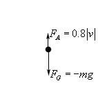
Because of the conventions the force due to gravity is negative and the force due to air resistance is positive. As set up, these forces have the correct sign and so the IVP is
\[mv' = - mg + 0.8\left| v \right|\hspace{0.25in}v\left( 0 \right) = 0\]The problem arises when you go to remove the absolute value bars. In order to do the problem they do need to be removed. This is where most of the students made their mistake. Because they had forgotten about the convention and the direction of motion they just dropped the absolute value bars to get.
\[mv' = - mg + 0.8v\hspace{0.25in}v\left( 0 \right) = 0\hspace{0.25in}\left( {{\mbox{incorrect IVP!!}}} \right)\]So, why is this incorrect? Well remember that the convention is that positive is upward. However in this case the object is moving downward and so \(v\) is negative! Upon dropping the absolute value bars the air resistance became a negative force and hence was acting in the downward direction!
To get the correct IVP recall that because \(v\) is negative then |\(v\)| = -\(v\). Using this, the air resistance becomes FA = -0.8\(v\) and despite appearances this is a positive force since the “-” cancels out against the velocity (which is negative) to get a positive force.
The correct IVP is then
\[mv' = - mg - 0.8v\hspace{0.25in}v\left( 0 \right) = 0\]Plugging in the mass gives
\[v' = - 9.8 - \frac{v}{{75}}\hspace{0.25in}v\left( 0 \right) = 0\]For the sake of completeness the velocity of the sky diver, at least until the parachute opens, which we didn’t include in this problem is.
\[v\left( t \right) = - 735 + 735{{\bf{e}}^{ - \frac{t}{{75}}}}\]This mistake was made in part because the students were in a hurry and weren’t paying attention, but also because they simply forgot about their convention and the direction of motion! Don’t fall into this mistake. Always pay attention to your conventions and what is happening in the problems.
Just to show you the difference here is the problem worked by assuming that down is positive.
Here are the forces that are acting on the sky diver
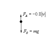
In this case the force due to gravity is positive since it’s a downward force and air resistance is an upward force and so needs to be negative. In this case since the motion is downward the velocity is positive so |\(v\)| = \(v\). The air resistance is then FA = -0.8\(v\). The IVP for this case is
\[mv' = mg - 0.8v\hspace{0.25in}v\left( 0 \right) = 0\]Plugging in the mass gives
\[v' = 9.8 - \frac{v}{{75}}\hspace{0.25in}v\left( 0 \right) = 0\]Solving this gives
\[v\left( t \right) = 735 - 735{{\bf{e}}^{ - \frac{t}{{75}}}}\]This is the same solution as the previous example, except that it’s got the opposite sign. This is to be expected since the conventions have been switched between the two examples.