Calculus III - Green's Theorem

Show Mobile Notice Show All Notes Hide All Notes

Mobile Notice

You appear to be on a device with a "narrow" screen width (i.e. you are probably on a mobile phone). Due to the nature of the mathematics on this site it is best views in landscape mode. If your device is not in landscape mode many of the equations will run off the side of your device (should be able to scroll to see them) and some of the menu items will be cut off due to the narrow screen width.

Section 16.7 : Green's Theorem

In this section we are going to investigate the relationship between certain kinds of line integrals (on closed paths) and double integrals.

Let’s start off with a simple (recall that this means that it doesn’t cross itself) closed curve $C$ and let $D$ be the region enclosed by the curve. Here is a sketch of such a curve and region.

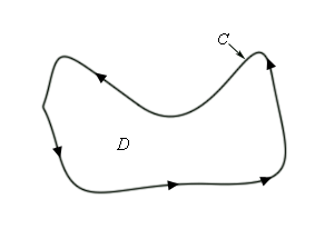
This is the 2D graph, without an axis system, of a generic curve. The curve is nearly rectangular except that the corners are rounded and the middle of the top “edge” dips down about 1/3 of the way into the interior. The curve is labeled C and there are arrow heads on the curve indicating that the curve is traced out in a counter clockwise direction. The region that is enclosed by the curve is labeled as D.

First, notice that because the curve is simple and closed there are no holes in the region $D$. Also notice that a direction has been put on the curve. We will use the convention here that the curve $C$ has a positive orientation if it is traced out in a counter-clockwise direction. Another way to think of a positive orientation (that will cover much more general curves as well see later) is that as we traverse the path following the positive orientation the region $D$ must always be on the left.

Given curves/regions such as this we have the following theorem.

Green’s Theorem

Let $C$ be a positively oriented, piecewise smooth, simple, closed curve and let $D$ be the region enclosed by the curve. If $P$ and $Q$ have continuous first order partial derivatives on $D$ then,

\[\int\limits_{C}{{Pdx\, + Qdy}} = \iint\limits_{D}{{\left( {\frac{{\partial Q}}{{\partial x}} - \frac{{\partial P}}{{\partial y}}} \right)\,dA}}\]

Before working some examples there are some alternate notations that we need to acknowledge. When working with a line integral in which the path satisfies the condition of Green’s Theorem we will often denote the line integral as,

\[\oint_{C}{{Pdx + Qdy}}\hspace{0.5in}{\mbox{or}}\hspace{0.25in}\mathop{\int\mkern-18.8mu \circlearrowleft}\limits_C {Pdx + Qdy} \]

Both of these notations do assume that $C$ satisfies the conditions of Green’s Theorem so be careful in using them.

Also, sometimes the curve $C$ is not thought of as a separate curve but instead as the boundary of some region $D$ and in these cases you may see $C$ denoted as $\partial D$.

Let’s work a couple of examples.

Example 1 Use Green’s Theorem to evaluate $ \displaystyle \oint_{C}{{xy\,dx + {x^2}{y^3}\,dy}}$ where $C$ is the triangle with vertices $\left( {0,0} \right)$, $\left( {1,0} \right)$, $\left( {1,2} \right)$ with positive orientation.

Show Solution

Let’s first sketch $C$ and $D$ for this case to make sure that the conditions of Green’s Theorem are met for $C$ and will need the sketch of $D$ to evaluate the double integral.

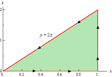
This is the 2D graph on a xy axis system of a triangle with vertices (0,0), (1,0) and (1,2). The top left edge of the triangle is given by y=2x. The bottom of the triangle is the x-axis and the left edge is the line x=1. The triangle has been shaded in and arrow heads on the triangle indicate that is traced out in a counter clockwise direction.

So, the curve does satisfy the conditions of Green’s Theorem and we can see that the following inequalities will define the region enclosed.

\[0 \le x \le 1\hspace{0.5in}0 \le y \le 2x\]

We can identify $P$ and $Q$ from the line integral. Here they are.

\[P = xy\hspace{0.5in}Q = {x^2}{y^3}\,\]

So, using Green’s Theorem the line integral becomes,

\[\begin{align*}\oint_{C}{{xy\,dx + {x^2}{y^3}\,dy}} & = \iint\limits_{D}{{2x{y^3} - x\,dA}}\\ & = \int_{{\,0}}^{{\,1}}{{\int_{{\,0}}^{{\,2x}}{{2x{y^3} - x\,dy}}\,dx}}\\ & = \int_{{\,0}}^{{\,1}}{{\left. {\left( {\frac{1}{2}x{y^4} - xy} \right)} \right|_0^{2x}\,dx}}\\ & = \int_{{\,0}}^{{\,1}}{{8{x^5} - 2{x^2}\,dx}}\\ & = \left. {\left( {\frac{4}{3}{x^6} - \frac{2}{3}{x^3}} \right)} \right|_0^1\\ & = \frac{2}{3}\end{align*}\]

Example 2 Evaluate $ \displaystyle \oint_{C}{{{y^3}\,dx - {x^3}\,dy}}$ where $C$ is the positively oriented circle of radius 2 centered at the origin.

Show Solution

Okay, a circle will satisfy the conditions of Green’s Theorem since it is closed and simple and so there really isn’t a reason to sketch it.

Let’s first identify $P$ and $Q$ from the line integral.

\[P = {y^3}\hspace{0.5in}Q = - {x^3}\]

Be careful with the minus sign on $Q$!

Now, using Green’s theorem on the line integral gives,

\[\oint_{C}{{{y^3}\,dx - {x^3}\,dy}} = \iint\limits_{D}{{ - 3{x^2} - 3{y^2}\,dA}}\]

where $D$ is a disk of radius 2 centered at the origin.

Since $D$ is a disk it seems like the best way to do this integral is to use polar coordinates. Here is the evaluation of the integral.

\[\begin{align*}\oint_{C}{{{y^3}\,dx - {x^3}\,dy}} & = - 3\iint\limits_{D}{{\left( {{x^2} + {y^2}} \right)\,dA}}\\ & = - 3\int_{{\,0}}^{{\,2\pi }}{{\int_{{\,0}}^{{\,2}}{{{r^3}\,dr}}\,d\theta }}\\ & = - 3\int_{{\,0}}^{{\,2\pi }}{{\left. {\frac{1}{4}{r^4}} \right|_0^2\,d\theta }}\\ & = - 3\int_{{\,0}}^{{\,2\pi }}{{4\,d\theta }}\\ & = - 24\pi \end{align*}\]

So, Green’s theorem, as stated, will not work on regions that have holes in them. However, many regions do have holes in them. So, let’s see how we can deal with those kinds of regions.

Let’s start with the following region. Even though this region doesn’t have any holes in it the arguments that we’re going to go through will be similar to those that we’d need for regions with holes in them, except it will be a little easier to deal with and write down.

$This is the 2D graph, without an axis system, of a generic curve. The curve is nearly rectangular except that the corners are rounded and the middle of the top “edge” dips down about 1/3 of the way into the interior. This is the same curve as was given at the start of the section except this time it has been vertically cut in the middle. The right portion of the original curve from the bottom cut point to the top cut point is labeled $C_{1}$ and has arrow heads indicating it is traced out in a counter clockwise direction. On the right side of the cut there is an arrow pointing downwards labeled $C_{3}$. The left portion of the original curve starting at the top cut point to the bottom cut point is labeled $C_{2}$ and has arrow heads indicating it is traced out in a counter clockwise direction. On the left side of the cut there is an arrow pointing upwards labeled $-C_{3}$. The right portion of the enclosed region is labeled $D_{1}$ and the left portion of the enclosed region is labeled $D_{2}$.$

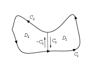
The region $D$ will be ${D_1} \cup {D_2}$ and recall that the symbol $ \cup $ is called the union and means that $D$ consists of both ${D_{_1}}$ and ${D_2}$. The boundary of ${D_{_1}}$ is ${C_1} \cup {C_3}$ while the boundary of ${D_2}$ is ${C_2} \cup \left( { - {C_3}} \right)$ and notice that both of these boundaries are positively oriented. As we traverse each boundary the corresponding region is always on the left. Finally, also note that we can think of the whole boundary, $C$, as,

\[C = \left( {{C_1} \cup {C_3}} \right) \cup \left( {{C_2} \cup \left( { - {C_3}} \right)} \right) = {C_1} \cup {C_2}\]

since both ${C_3}$ and $ - {C_3}$ will “cancel” each other out.

Now, let’s start with the following double integral and use a basic property of double integrals to break it up.

\[\iint\limits_{D}{{\left( {{Q_x} - {P_y}} \right)\,dA}} = \iint\limits_{{{D_1} \cup {D_2}}}{{\left( {{Q_x} - {P_y}} \right)\,dA}} = \iint\limits_{{{D_1}}}{{\left( {{Q_x} - {P_y}} \right)\,dA}} + \iint\limits_{{{D_2}}}{{\left( {{Q_x} - {P_y}} \right)\,dA}}\]

Next, use Green’s theorem on each of these and again use the fact that we can break up line integrals into separate line integrals for each portion of the boundary.

\[\begin{align*}\iint\limits_{D}{{\left( {{Q_x} - {P_y}} \right)\,dA}} & = \iint\limits_{{{D_1}}}{{\left( {{Q_x} - {P_y}} \right)\,dA}} + \iint\limits_{{{D_2}}}{{\left( {{Q_x} - {P_y}} \right)\,dA}}\\ & = \oint\limits_{{{C_1} \cup {C_3}}}{{Pdx + Qdy}} + \oint\limits_{{{C_2} \cup \left( { - {C_3}} \right)}}{{Pdx + Qdy}}\\ & = \oint\limits_{{{C_1}}}{{Pdx + Qdy}} + \oint\limits_{{{C_3}}}{{Pdx + Qdy}} + \oint\limits_{{{C_2}}}{{Pdx + Qdy}} + \oint\limits_{{ - {C_3}}}{{Pdx + Qdy}}\end{align*}\]

Next, we’ll use the fact that,

\[\oint\limits_{{ - {C_3}}}{{Pdx + Qdy}} = - \oint\limits_{{{C_3}}}{{Pdx + Qdy}}\]

Recall that changing the orientation of a curve with line integrals with respect to $x$ and/or $y$ will simply change the sign on the integral. Using this fact we get,

\[\begin{align*}\iint\limits_{D}{{\left( {{Q_x} - {P_y}} \right)\,dA}} & = \oint\limits_{{{C_1}}}{{Pdx + Qdy}} + \oint\limits_{{{C_3}}}{{Pdx + Qdy}} + \oint\limits_{{{C_2}}}{{Pdx + Qdy}} - \oint\limits_{{{C_3}}}{{Pdx + Qdy}}\\ & = \oint\limits_{{{C_1}}}{{Pdx + Qdy}} + \oint\limits_{{{C_2}}}{{Pdx + Qdy}}\end{align*}\]

Finally, put the line integrals back together and we get,

\[\begin{align*}\iint\limits_{D}{{\left( {{Q_x} - {P_y}} \right)\,dA}} & = \oint\limits_{{{C_1}}}{{Pdx + Qdy}} + \oint\limits_{{{C_2}}}{{Pdx + Qdy}}\\ & = \oint\limits_{{{C_1} \cup {C_2}}}{{Pdx + Qdy}}\\ & = \oint\limits_{C}{{Pdx + Qdy}}\end{align*}\]

So, what did we learn from this? If you think about it this was just a lot of work and all we got out of it was the result from Green’s Theorem which we already knew to be true. What this exercise has shown us is that if we break a region up as we did above then the portion of the line integral on the pieces of the curve that are in the middle of the region (each of which are in the opposite direction) will cancel out. This idea will help us in dealing with regions that have holes in them.

To see this let’s look at a ring.

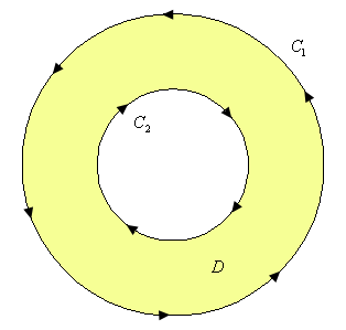
$This is the 2D graph, without an axis system, of ring. The outer radius of the disk is labeled $C_{1}$ and has arrow heads indicating it is traced out in a counter clockwise direction. The inner radius of the disk is labeled $C_{2}$ and has arrow heads indicating it is traced out in a clockwise direction. The ring enclosed by the two radii is labeled D.$

Notice that both of the curves are oriented positively since the region $D$ is on the left side as we traverse the curve in the indicated direction. Note as well that the curve ${C_2}$ seems to violate the original definition of positive orientation. We originally said that a curve had a positive orientation if it was traversed in a counter-clockwise direction. However, this was only for regions that do not have holes. For the boundary of the hole this definition won’t work and we need to resort to the second definition that we gave above.

Now, since this region has a hole in it we will apparently not be able to use Green’s Theorem on any line integral with the curve $C = {C_1} \cup {C_2}$. However, if we cut the disk in half and rename all the various portions of the curves we get the following sketch.

$This is the same ring as above except it has been cut horizontally through the center. The top portion of the outer radius is labeled $C_{1}$ and has arrow heads on the curve indicating that the curve is traced out in a counter clockwise direction. On the top of the left cut is an arrow pointing right labeled $C_{5}$. The top portion of the inner radius is labeled $C_{2}$ and has arrow heads on the curve indicating that the curve is traced out in a clockwise direction. On the top of the right cut is an arrow pointing right labeled $C_{6}$. The upper portion of the enclosed ring is labeled $D_{1}$. The bottom portion of the outer radius is labeled $C_{4}$ and has arrow heads on the curve indicating that the curve is traced out in a counter clockwise direction. On the bottom of the left cut is an arrow pointing left labeled $-C_{5}$. The bottom portion of the inner radius is labeled $C_{3}$ and has arrow heads on the curve indicating that the curve is traced out in a clockwise direction. On the bottom of the right cut is an arrow pointing left labeled $-C_{6}$. The lower portion of the enclosed ring is labeled $D_{2}$.$

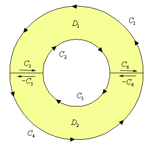
The boundary of the upper portion (${D_{_1}}$)of the disk is ${C_1} \cup {C_2} \cup {C_5} \cup {C_6}$ and the boundary on the lower portion (${D_2}$)of the disk is ${C_3} \cup {C_4} \cup \left( { - {C_5}} \right) \cup \left( { - {C_6}} \right)$. Also notice that we can use Green’s Theorem on each of these new regions since they don’t have any holes in them. This means that we can do the following,

\[\begin{align*}\iint\limits_{D}{{\left( {{Q_x} - {P_y}} \right)\,dA}} & = \iint\limits_{{{D_1}}}{{\left( {{Q_x} - {P_y}} \right)\,dA}} + \iint\limits_{{{D_2}}}{{\left( {{Q_x} - {P_y}} \right)\,dA}}\\ & = \oint_{{{C_1} \cup {C_2} \cup {C_5} \cup {C_6}}}{{Pdx + Qdy}} + \oint_{{{C_3} \cup {C_4} \cup \left( { - {C_5}} \right) \cup \left( { - {C_6}} \right)}}{{Pdx + Qdy}}\end{align*}\]

Now, we can break up the line integrals into line integrals on each piece of the boundary. Also recall from the work above that boundaries that have the same curve, but opposite direction will cancel. Doing this gives,

But at this point we can add the line integrals back up as follows,

\[\begin{align*}\iint\limits_{D}{{\left( {{Q_x} - {P_y}} \right)\,dA}} & = \oint_{{{C_1} \cup {C_2} \cup {C_3} \cup {C_4}}}{{Pdx + Qdy}}\\ & = \oint_{C}{{Pdx + Qdy}}\end{align*}\]

The end result of all of this is that we could have just used Green’s Theorem on the disk from the start even though there is a hole in it. This will be true in general for regions that have holes in them.

Let’s take a look at an example.

Example 3 Evaluate $ \displaystyle \oint_{C}{{{y^3}\,dx - {x^3}\,dy}}$ where $C$ are the two circles of radius 2 and radius 1 centered at the origin with positive orientation.

Show Solution

Notice that this is the same line integral as we looked at in the second example and only the curve has changed. In this case the region $D$ will now be the region between these two circles and that will only change the limits in the double integral so we’ll not put in some of the details here.

Here is the work for this integral.

\[\begin{align*}\oint_{C}{{{y^3}\,dx - {x^3}\,dy}} & = - 3\iint\limits_{D}{{\left( {{x^2} + {y^2}} \right)\,dA}}\\ & = - 3\int_{{\,0}}^{{\,2\pi }}{{\int_{{\,1}}^{{\,2}}{{{r^3}\,dr}}\,d\theta }}\\ & = - 3\int_{{\,0}}^{{\,2\pi }}{{\left. {\frac{1}{4}{r^4}} \right|_1^2\,d\theta }}\\ & = - 3\int_{{\,0}}^{{\,2\pi }}{{\frac{{15}}{4}\,d\theta }}\\ & = - \frac{{45\pi }}{2}\end{align*}\]

We will close out this section with an interesting application of Green’s Theorem. Recall that we can determine the area of a region $D$ with the following double integral.

\[A = \iint\limits_{D}{{dA}}\]

Let’s think of this double integral as the result of using Green’s Theorem. In other words, let’s assume that

\[{Q_x} - {P_y} = 1\]

and see if we can get some functions $P$ and $Q$ that will satisfy this.

There are many functions that will satisfy this. Here are some of the more common functions.

\[\begin{array}{c}\begin{array}{l}P = 0 & & \\Q = x\end{array}&\begin{array}{l}P = - y & & \\\,\,Q = 0\end{array}&\begin{array}{l}P = - \frac{y}{2}\\\,\,Q = \frac{x}{2}\end{array}\end{array}\]

Then, if we use Green’s Theorem in reverse we see that the area of the region $D$ can also be computed by evaluating any of the following line integrals.

\[A = \oint\limits_{C}{{x\,dy}} = - \,\oint\limits_{C}{{y\,dx}} = \frac{1}{2}\oint\limits_{C}{{x\,dy - y\,dx}}\]

where $C$ is the boundary of the region $D$.

Let’s take a quick look at an example of this.

Example 4 Use Green’s Theorem to find the area of a disk of radius $a$.

Show Solution

We can use either of the integrals above, but the third one is probably the easiest. So,

\[A = \frac{1}{2}\oint\limits_{C}{{x\,dy - y\,dx}}\]

where $C$ is the circle of radius $a$. So, to do this we’ll need a parameterization of $C$. This is,

\[x = a\cos t\hspace{0.25in}y = a\sin t\hspace{0.25in}0 \le t \le 2\pi \]

The area is then,

\[\begin{align*}A = \frac{1}{2}\oint\limits_{C}{{x\,dy - y\,dx}}\\ & = \frac{1}{2}\left( {\int_{{\,0}}^{{\,2\pi }}{{a\cos t\left( {a\cos t} \right)\,dt}} - \int_{{\,0}}^{{\,2\pi }}{{a\sin t\left( { - a\sin t} \right)\,dt}}} \right)\\ & = \frac{1}{2}\int_{{\,0}}^{{\,2\pi }}{{{a^2}{{\cos }^2}t + {a^2}{{\sin }^2}t\,dt}}\\ & = \frac{1}{2}\int_{{\,0}}^{{\,2\pi }}{{{a^2}dt}}\\ & = \pi {a^2}\end{align*}\]