Section 8.1 : Arc Length
In this section we are going to look at computing the arc length of a function. Because it’s easy enough to derive the formulas that we’ll use in this section we will derive one of them and leave the other to you to derive.
We want to determine the length of the continuous function \(y = f\left( x \right)\) on the interval \(\left[ {a,b} \right]\). We’ll also need to assume that the derivative is continuous on \(\left[ {a,b} \right]\).
Initially we’ll need to estimate the length of the curve. We’ll do this by dividing the interval up into \(n\) equal subintervals each of width \(\Delta x\) and we’ll denote the point on the curve at each point by Pi. We can then approximate the curve by a series of straight lines connecting the points. Here is a sketch of this situation for \(n = 9\).
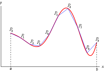
Now denote the length of each of these line segments by \(\left| {{P_{i - 1}}\,\,{P_i}} \right|\) and the length of the curve will then be approximately,
\[L \approx \sum\limits_{i = 1}^n {\left| {{P_{i - 1}}\,\,{P_i}} \right|} \]and we can get the exact length by taking \(n\) larger and larger. In other words, the exact length will be,
\[L = \mathop {\lim }\limits_{n \to \infty } \sum\limits_{i = 1}^n {\left| {{P_{i - 1}}\,\,{P_i}} \right|} \]Now, let’s get a better grasp on the length of each of these line segments. First, on each segment let’s define \(\Delta {y_i} = {y_i} - {y_{i - 1}} = f\left( {{x_i}} \right) - f\left( {{x_{i - 1}}} \right)\). We can then compute directly the length of the line segments as follows.
\[\left| {{P_{i - 1}}\,\,{P_i}} \right| = \sqrt {{{\left( {{x_i} - {x_{i - 1}}} \right)}^2} + {{\left( {{y_i} - {y_{i - 1}}} \right)}^2}} = \sqrt {\Delta {x^2} + \Delta y_i^2} \]By the Mean Value Theorem we know that on the interval \(\left[ {{x_{i - 1}},{x_i}} \right]\) there is a point \(x_i^*\) so that,
\[\begin{align*}f\left( {{x_i}} \right) - f\left( {{x_{i - 1}}} \right) & = f'\left( {x_i^*} \right)\left( {{x_i} - {x_{i - 1}}} \right)\\ & \Delta {y_i} = f'\left( {x_i^*} \right)\Delta x\end{align*}\]Therefore, the length can now be written as,
\[\begin{align*}\left| {{P_{i - 1}}\,\,{P_i}} \right| & = \sqrt {{{\left( {{x_i} - {x_{i - 1}}} \right)}^2} + {{\left( {{y_i} - {y_{i - 1}}} \right)}^2}} \\ & = \sqrt {\Delta {x^2} + {{\left[ {f'\left( {x_i^*} \right)} \right]}^2}\Delta {x^2}} \\ & = \sqrt {1 + {{\left[ {f'\left( {x_i^*} \right)} \right]}^2}} \,\,\,\Delta x\end{align*}\]The exact length of the curve is then,
\[\begin{align*}L & = \mathop {\lim }\limits_{n \to \infty } \sum\limits_{i = 1}^n {\left| {{P_{i - 1}}\,\,{P_i}} \right|} \\ & = \mathop {\lim }\limits_{n \to \infty } \sum\limits_{i = 1}^n {\sqrt {1 + {{\left[ {f'\left( {x_i^*} \right)} \right]}^2}} \,\,\,\Delta x} \end{align*}\]However, using the definition of the definite integral, this is nothing more than,
\[L = \int_{{\,a}}^{{\,b}}{{\sqrt {1 + {{\left[ {f'\left( x \right)} \right]}^2}} \,dx}}\]A slightly more convenient notation (in our opinion anyway) is the following.
\[L = \int_{{\,a}}^{{\,b}}{{\sqrt {1 + {{\left( {\frac{{dy}}{{dx}}} \right)}^2}} \,dx}}\]In a similar fashion we can also derive a formula for \(x = h\left( y \right)\) on \(\left[ {c,d} \right]\). This formula is,
\[L = \int_{{\,c}}^{{\,d}}{{\sqrt {1 + {{\left[ {h'\left( y \right)} \right]}^2}} \,dy}} = \int_{{\,c}}^{{\,d}}{{\sqrt {1 + {{\left( {\frac{{dx}}{{dy}}} \right)}^2}} \,dy}}\]Again, the second form is probably a little more convenient.
Note the difference in the derivative under the square root! Don’t get too confused. With one we differentiate with respect to \(x\) and with the other we differentiate with respect to \(y\). One way to keep the two straight is to notice that the differential in the “denominator” of the derivative will match up with the differential in the integral. This is one of the reasons why the second form is a little more convenient.
Before we work any examples we need to make a small change in notation. Instead of having two formulas for the arc length of a function we are going to reduce it, in part, to a single formula.
From this point on we are going to use the following formula for the length of the curve.
Arc Length Formula(s)
where,
\[\begin{array}{*{20}{l}}\begin{aligned}ds & = \sqrt {1 + {{\left( {\frac{{dy}}{{dx}}} \right)}^2}} \,dx\,\hspace{0.25in}{\mbox{if }}y = f\left( x \right),\,\,a \le x \le b\\ ds & = \sqrt {1 + {{\left( {\frac{{dx}}{{dy}}} \right)}^2}} \,dy\,\hspace{0.25in}{\mbox{if }}x = h\left( y \right),\,\,c \le y \le d\end{aligned}\end{array}\]Note that no limits were put on the integral as the limits will depend upon the \(ds\) that we’re using. Using the first \(ds\) will require \(x\) limits of integration and using the second \(ds\) will require \(y\) limits of integration.
Thinking of the arc length formula as a single integral with different ways to define \(ds\) will be convenient when we run across arc lengths in future sections. Also, this \(ds\) notation will be a nice notation for the next section as well.
Now that we’ve derived the arc length formula let’s work some examples.
In this case we’ll need to use the first \(ds\) since the function is in the form \(y = f\left( x \right)\). So, let’s get the derivative out of the way.
\[\frac{{dy}}{{dx}} = \frac{{\sec x\tan x}}{{\sec x}} = \tan x\hspace{0.5in}{\left( {\frac{{dy}}{{dx}}} \right)^2} = {\tan ^2}x\]Let’s also get the root out of the way since there is often simplification that can be done and there’s no reason to do that inside the integral.
\[\sqrt {1 + {{\left( {\frac{{dy}}{{dx}}} \right)}^2}} = \sqrt {1 + {{\tan }^2}x} = \sqrt {{{\sec }^2}x} = \left| {\sec x} \right| = \sec x\]Note that we could drop the absolute value bars here since secant is positive in the range given.
The arc length is then,
\[\begin{align*}L & = \int_{{\,0}}^{{\,\frac{\pi }{4}}}{{\sec x\,dx}}\\ & = \left. {\ln \left| {\sec x + \tan x} \right|} \right|_0^{\frac{\pi }{4}}\\ & = \ln \left( {\sqrt 2 + 1} \right)\end{align*}\]There is a very common mistake that students make in problems of this type. Many students see that the function is in the form \(x = h\left( y \right)\) and they immediately decide that it will be too difficult to work with it in that form so they solve for \(y\) to get the function into the form \(y = f\left( x \right)\). While that can be done here it will lead to a messier integral for us to deal with.
Sometimes it’s just easier to work with functions in the form \(x = h\left( y \right)\). In fact, if you can work with functions in the form \(y = f\left( x \right)\) then you can work with functions in the form \(x = h\left( y \right)\). There really isn’t a difference between the two so don’t get excited about functions in the form \(x = h\left( y \right)\).
Let’s compute the derivative and the root.
\[\frac{{dx}}{{dy}} = {\left( {y - 1} \right)^{\frac{1}{2}}}\hspace{0.5in} \Rightarrow \hspace{0.5in}\sqrt {1 + {{\left( {\frac{{dx}}{{dy}}} \right)}^2}} = \sqrt {1 + y - 1} = \sqrt y \]As you can see keeping the function in the form \(x = h\left( y \right)\) is going to lead to a very easy integral. To see what would happen if we tried to work with the function in the form \(y = f\left( x \right)\) see the next example.
Let’s get the length.
\[\begin{align*}L & = \int_{{\,1}}^{{\,4}}{{\sqrt y \,dy}}\\ & = \left. {\frac{2}{3}{y^{\frac{3}{2}}}} \right|_1^4\\ & = \frac{{14}}{3}\end{align*}\]As noted in the last example we really do have a choice as to which \(ds\) we use. Provided we can get the function in the form required for a particular \(ds\) we can use it. However, as also noted above, there will often be a significant difference in difficulty in the resulting integrals. Let’s take a quick look at what would happen in the previous example if we did put the function into the form \(y = f\left( x \right)\).
In this case the function and its derivative would be,
\[y = {\left( {\frac{{3x}}{2}} \right)^{\frac{2}{3}}} + 1\hspace{0.5in}\hspace{0.25in}\frac{{dy}}{{dx}} = {\left( {\frac{{3x}}{2}} \right)^{ - \frac{1}{3}}}\]The root in the arc length formula would then be.
\[\sqrt {1 + {{\left( {\frac{{dy}}{{dx}}} \right)}^2}} = \sqrt {1 + \frac{1}{{{{\left( {\frac{{3x}}{2}} \right)}^{\frac{2}{3}}}}}} = \sqrt {\frac{{{{\left( {\frac{{3x}}{2}} \right)}^{\frac{2}{3}}} + 1}}{{{{\left( {\frac{{3x}}{2}} \right)}^{\frac{2}{3}}}}}} = \frac{{\sqrt {{{\left( {\frac{{3x}}{2}} \right)}^{\frac{2}{3}}} + 1} }}{{{{\left( {\frac{{3x}}{2}} \right)}^{\frac{1}{3}}}}}\]All the simplification work above was just to put the root into a form that will allow us to do the integral.
Now, before we write down the integral we’ll also need to determine the limits. This particular \(ds\) requires \(x\) limits of integration and we’ve got \(y\) limits. They are easy enough to get however. Since we know \(x\) as a function of \(y\) all we need to do is plug in the original \(y\) limits of integration and get the \(x\) limits of integration. Doing this gives,
\[0 \le x \le \frac{2}{3}{\left( 3 \right)^{\frac{3}{2}}}\]Not easy limits to deal with, but there they are.
Let’s now write down the integral that will give the length.
\[L = \int_{{\,0}}^{{\,\frac{2}{3}{{\left( 3 \right)}^{\frac{3}{2}}}}}{{\frac{{\sqrt {{{\left( {\frac{{3x}}{2}} \right)}^{\frac{2}{3}}} + 1} }}{{{{\left( {\frac{{3x}}{2}} \right)}^{\frac{1}{3}}}}}\,dx}}\]That’s a really unpleasant looking integral. It can be evaluated however using the following substitution.
\[u = {\left( {\frac{{3x}}{2}} \right)^{\frac{2}{3}}} + 1\hspace{0.5in}\hspace{0.25in}du = {\left( {\frac{{3x}}{2}} \right)^{ - \frac{1}{3}}}dx\] \[\begin{align*}x & = 0 & \hspace{0.25in} \Rightarrow \hspace{0.5in}u = 1\\ x & = \frac{2}{3}{\left( 3 \right)^{\frac{3}{2}}} & \hspace{0.25in} \Rightarrow \hspace{0.5in}u = 4\end{align*}\]Using this substitution the integral becomes,
\[\begin{align*}L & = \int_{{\,1}}^{{\,4}}{{\sqrt u \,du}}\\ & = \left. {\frac{2}{3}{u^{\frac{3}{2}}}} \right|_1^4\\ & = \frac{{14}}{3}\end{align*}\]So, we got the same answer as in the previous example. Although that shouldn’t really be all that surprising since we were dealing with the same curve.
From a technical standpoint the integral in the previous example was not that difficult. It was just a Calculus I substitution. However, from a practical standpoint the integral was significantly more difficult than the integral we evaluated in Example 2. So, the moral of the story here is that we can use either formula (provided we can get the function in the correct form of course) however one will often be significantly easier to actually evaluate.
Okay, let’s work one more example.
We’ll use the second \(ds\) for this one as the function is already in the correct form for that one. Also, the other \(ds\) would again lead to a particularly difficult integral. The derivative and root will then be,
\[\frac{{dx}}{{dy}} = y\hspace{0.5in} \Rightarrow \hspace{0.5in}\sqrt {1 + {{\left( {\frac{{dx}}{{dy}}} \right)}^2}} = \sqrt {1 + {y^2}} \]Before writing down the length notice that we were given \(x\) limits and we will need \(y\) limits for this \(ds\). With the assumption that \(y\) is positive these are easy enough to get. All we need to do is plug \(x\) into our equation and solve for \(y\). Doing this gives,
\[0 \le y \le 1\]The integral for the arc length is then,
\[L = \int_{{\,0}}^{{\,1}}{{\sqrt {1 + {y^2}} \,dy}}\]This integral will require the following trig substitution.
\[y = \tan \theta \hspace{0.5in}dy = {\sec ^2}\theta \,d\theta \] \[\begin{align*}y & = 0 & \hspace{0.25in} \Rightarrow \hspace{0.25in}0 = \tan \theta \hspace{0.25in} \Rightarrow \hspace{0.25in}\theta = 0 \,\,\, \\ y & = 1 & \hspace{0.25in} \Rightarrow \hspace{0.25in}1 = \tan \theta \hspace{0.25in} \Rightarrow \hspace{0.25in}\theta = \frac{\pi }{4}\end{align*}\] \[\sqrt {1 + {y^2}} = \sqrt {1 + {{\tan }^2}\theta } = \sqrt {{{\sec }^2}\theta } = \left| {\sec \theta } \right| = \sec \theta \]The length is then,
\[\begin{align*}L & = \int_{{\,0}}^{{\,\frac{\pi }{4}}}{{{{\sec }^3}\theta \,d\theta }}\\ & = \left. {\frac{1}{2}\left( {\sec \theta \tan \theta + \ln \left| {\sec \theta + \tan \theta } \right|} \right)} \right|_0^{\frac{\pi }{4}}\\ & = \frac{1}{2}\left( {\sqrt 2 + \ln \left( {1 + \sqrt 2 } \right)} \right)\end{align*}\]The first couple of examples ended up being fairly simple Calculus I substitutions. However, as this last example had shown we can end up with trig substitutions as well for these integrals.