Section 2.3 : One-Sided Limits
In the final two examples in the previous section we saw two limits that did not exist. However, the reason for each of the limits not existing was different for each of the examples.
We saw that
\[\mathop {\lim }\limits_{t \to 0} \,\,\cos \left( {\frac{\pi }{t}} \right)\]did not exist because the function did not settle down to a single value as \(t\) approached \(t = 0\). The closer to \(t = 0\) we moved the more wildly the function oscillated and in order for a limit to exist the function must settle down to a single value.
However, we saw that
\[\mathop {\lim }\limits_{t \to 0} H\left( t \right)\hspace{0.25in}{\mbox{where,}}\hspace{0.25in}H\left( t \right) = \left\{ \begin{array}{ll}0 & {\mbox{if }}t < 0\\ 1 & {\mbox{if }}t \ge 0\end{array} \right.\]did not exist not because the function didn’t settle down to a single number as we moved in towards \(t = 0\), but instead because it settled into two different numbers depending on which side of \(t = 0\) we were on.
In this case the function was a very well-behaved function, unlike the first function. The only problem was that, as we approached \(t = 0\), the function was moving in towards different numbers on each side. We would like a way to differentiate between these two examples.
We do this with one-sided limits. As the name implies, with one-sided limits we will only be looking at one side of the point in question. Here are the definitions for the two one sided limits.
Right-handed limit
We say
\[\mathop {\lim }\limits_{x \to {a^ + }} f\left( x \right) = L\]provided we can make \(f\left( x \right)\) as close to \(L\) as we want for all \(x\) sufficiently close to \(a\) with \(x > a\) without actually letting \(x\) be \(a\).
Left-handed limit
We say
\[\mathop {\lim }\limits_{x \to {a^ - }} f\left( x \right) = L\]provided we can make \(f\left( x \right)\) as close to \(L\) as we want for all \(x\) sufficiently close to \(a\) with \(x < a\) without actually letting \(x\) be \(a\).
Note that the change in notation is very minor and in fact might be missed if you aren’t paying attention. The only difference is the bit that is under the “lim” part of the limit. For the right-handed limit we now have \(x \to {a^ + }\)(note the “+”) which means that we know will only look at \(x > a\). Likewise, for the left-handed limit we have \(x \to {a^ - }\)(note the “-”) which means that we will only be looking at \(x < a\).
Also, note that as with the “normal” limit (i.e. the limits from the previous section) we still need the function to settle down to a single number in order for the limit to exist. The only difference this time is that the function only needs to settle down to a single number on either the right side of \(x = a\) or the left side of \(x = a\) depending on the one‑sided limit we’re dealing with.
So, when we are looking at limits it’s now important to pay very close attention to see whether we are doing a normal limit or one of the one-sided limits. Let’s now take a look at the some of the problems from the last section and look at one-sided limits instead of the normal limit.
To remind us what this function looks like here’s the graph.
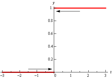
So, we can see that if we stay to the right of \(t = 0\) (i.e. \(t > 0\)) then the function is moving in towards a value of 1 as we get closer and closer to \(t = 0\), but staying to the right. We can therefore say that the right-handed limit is,
\[\mathop {\lim }\limits_{t \to {0^ + }} H\left( t \right) = 1\]Likewise, if we stay to the left of \(t = 0\) (i.e \(t < 0\)) the function is moving in towards a value of 0 as we get closer and closer to \(t = 0\), but staying to the left. Therefore, the left-handed limit is,
\[\mathop {\lim }\limits_{t \to {0^ - }} H\left( t \right) = 0\]In this example we do get one-sided limits even though the normal limit itself doesn’t exist.
From the graph of this function shown below,
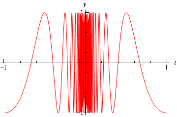
we can see that both of the one-sided limits suffer the same problem that the normal limit did in the previous section. The function does not settle down to a single number on either side of \(t = 0\). Therefore, neither the left-handed nor the right-handed limit will exist in this case.
So, one-sided limits don’t have to exist just as normal limits aren’t guaranteed to exist.
Let’s take a look at another example from the previous section.
So, as we’ve done with the previous two examples, let’s remind ourselves of the graph of this function.
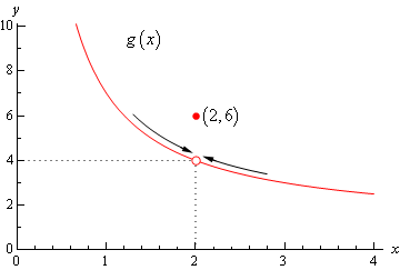
In this case regardless of which side of \(x = 2\) we are on the function is always approaching a value of 4 and so we get,
\[\mathop {\lim }\limits_{x \to {2^ + }} g\left( x \right) = 4\hspace{0.25in}\hspace{0.25in}\hspace{0.25in}\mathop {\lim }\limits_{x \to {2^ - }} g\left( x \right) = 4\]Note that one-sided limits do not care about what’s happening at the point any more than normal limits do. They are still only concerned with what is going on around the point. The only real difference between one-sided limits and normal limits is the range of \(x\)’s that we look at when determining the value of the limit.
Now let’s take a look at the first and last example in this section to get a very nice fact about the relationship between one-sided limits and normal limits. In the last example the one-sided limits as well as the normal limit existed and all three had a value of 4. In the first example the two one-sided limits both existed, but did not have the same value and the normal limit did not exist.
The relationship between one-sided limits and normal limits can be summarized by the following fact.
Fact
Given a function f(x) if,
\[\mathop {\lim }\limits_{x \to {a^ + }} f\left( x \right) = \mathop {\lim }\limits_{x \to {a^ - }} f\left( x \right) = L\]then the normal limit will exist and
\[\mathop {\lim }\limits_{x \to a} f\left( x \right) = L\]Likewise, if
\[\mathop {\lim }\limits_{x \to a} f\left( x \right) = L\]then,
\[\mathop {\lim }\limits_{x \to {a^ + }} f\left( x \right) = \mathop {\lim }\limits_{x \to {a^ - }} f\left( x \right) = L\]This fact can be turned around to also say that if the two one-sided limits have different values, i.e.,
\[\mathop {\lim }\limits_{x \to {a^ + }} f\left( x \right) \ne \mathop {\lim }\limits_{x \to {a^ - }} f\left( x \right)\]then the normal limit will not exist.
This should make some sense. If the normal limit did exist then by the fact the two one-sided limits would have to exist and have the same value by the above fact. So, if the two one-sided limits have different values (or don’t even exist) then the normal limit simply can’t exist.
Let’s take a look at one more example to make sure that we’ve got all the ideas about limits down that we’ve looked at in the last couple of sections.
compute each of the following.
- \(f( - 4)\)
- \(\mathop {\lim }\limits_{x \to - {4^ - }} f\left( x \right)\)
- \(\mathop {\lim }\limits_{x \to - {4^ + }} f\left( x \right)\)
- \(\mathop {\lim }\limits_{x \to - 4} f\left( x \right)\)
- \(f\left( 1 \right)\)
- \(\mathop {\lim }\limits_{x \to {1^ - }} f\left( x \right)\)
- \(\mathop {\lim }\limits_{x \to {1^ + }} f\left( x \right)\)
- \(\mathop {\lim }\limits_{x \to 1} f\left( x \right)\)
- \(f\left( 6 \right)\)
- \(\mathop {\lim }\limits_{x \to {6^ - }} f\left( x \right)\)
- \(\mathop {\lim }\limits_{x \to {6^ + }} f\left( x \right)\)
- \(\mathop {\lim }\limits_{x \to 6} f\left( x \right)\)
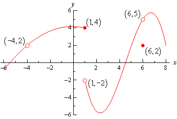
a\(f( - 4)\) doesn’t exist. There is no closed dot for this value of \(x\) and so the function doesn’t exist at this point.
b\(\mathop {\lim }\limits_{x \to - {4^ - }} f\left( x \right) = 2\) The function is approaching a value of 2 as \(x\) moves in towards -4 from the left.
c\(\mathop {\lim }\limits_{x \to - {4^ + }} f\left( x \right) = 2\) The function is approaching a value of 2 as \(x\) moves in towards -4 from the right.
d\(\mathop {\lim }\limits_{x \to - 4} f\left( x \right) = 2\) We can do this one of two ways. Either we can use the fact here and notice that the two one-sided limits are the same and so the normal limit must exist and have the same value as the one-sided limits or just get the answer from the graph.
Also recall that a limit can exist at a point even if the function doesn’t exist at that point.
e\(f\left( 1 \right) = 4\). The function will take on the \(y\) value where the closed dot is.
f\(\mathop {\lim }\limits_{x \to {1^ - }} f\left( x \right) = 4\) The function is approaching a value of 4 as \(x\) moves in towards 1 from the left.
g\(\mathop {\lim }\limits_{x \to {1^ + }} f\left( x \right) = - 2\) The function is approaching a value of -2 as \(x\) moves in towards 1 from the right. Remember that the limit does NOT care about what the function is actually doing at the point, it only cares about what the function is doing around the point. In this case, always staying to the right of \(x = 1\), the function is approaching a value of -2 and so the limit is -2. The limit is not 4, as that is value of the function at the point and again the limit doesn’t care about that!
h\(\mathop {\lim }\limits_{x \to 1} f\left( x \right)\) doesn’t exist. The two one-sided limits both exist, however they are different and so the normal limit doesn’t exist.
i\(f\left( 6 \right) = 2\). The function will take on the \(y\) value where the closed dot is.
j\(\mathop {\lim }\limits_{x \to {6^ - }} f\left( x \right) = 5\) The function is approaching a value of 5 as \(x\) moves in towards 6 from the left.
k\(\mathop {\lim }\limits_{x \to {6^ + }} f\left( x \right) = 5\) The function is approaching a value of 5 as \(x\) moves in towards 6 from the right.
l\(\mathop {\lim }\limits_{x \to 6} f\left( x \right) = 5\) Again, we can use either the graph or the fact to get this. Also, once more remember that the limit doesn’t care what is happening at the point and so it’s possible for the limit to have a different value than the function at a point. When dealing with limits we’ve always got to remember that limits simply do not care about what the function is doing at the point in question. Limits are only concerned with what the function is doing around the point.
Hopefully over the last couple of sections you’ve gotten an idea on how limits work and what they can tell us about functions. Some of these ideas will be important in later sections so it’s important that you have a good grasp on them.