Section 4.5 : The Shape of a Graph, Part I
In the previous section we saw how to use the derivative to determine the absolute minimum and maximum values of a function. However, there is a lot more information about a graph that can be determined from the first derivative of a function. We will start looking at that information in this section. The main idea we’ll be looking at in this section will be identifying all the relative extrema of a function.
Let’s start this section off by revisiting a familiar topic from the previous chapter. Let’s suppose that we have a function, \(f\left( x \right)\). We know from our work in the previous chapter that the first derivative, \(f'\left( x \right)\), is the rate of change of the function. We used this idea to identify where a function was increasing, decreasing or not changing.
Before reviewing this idea let’s first write down the mathematical definition of increasing and decreasing. We all know what the graph of an increasing/decreasing function looks like but sometimes it is nice to have a mathematical definition as well. Here it is.
Definition
- Given any \({x_1}\) and \({x_2}\) from an interval \(I\) with \({x_1} < {x_2}\) if \(f\left( {{x_1}} \right) < f\left( {{x_2}} \right)\) then \(f\left( x \right)\) is increasing on \(I\).
- Given any \({x_1}\) and \({x_2}\) from an interval \(I\) with \({x_1} < {x_2}\) if \(f\left( {{x_1}} \right) > f\left( {{x_2}} \right)\) then \(f\left( x \right)\) is decreasing on \(I\).
This definition will actually be used in the proof of the next fact in this section.
Now, recall that in the previous chapter we constantly used the idea that if the derivative of a function was positive at a point then the function was increasing at that point and if the derivative was negative at a point then the function was decreasing at that point. We also used the fact that if the derivative of a function was zero at a point then the function was not changing at that point. We used these ideas to identify the intervals in which a function is increasing and decreasing.
The following fact summarizes up what we were doing in the previous chapter.
Fact
- If \(f'\left( x \right) > 0\) for every \(x\) on some interval \(I\), then \(f\left( x \right)\) is increasing on the interval.
- If \(f'\left( x \right) < 0\) for every \(x\) on some interval \(I\), then \(f\left( x \right)\) is decreasing on the interval.
- If \(f'\left( x \right) = 0\) for every \(x\) on some interval \(I\), then \(f\left( x \right)\) is constant on the interval.
The proof of this fact is in the Proofs From Derivative Applications section of the Extras chapter.
Let’s take a look at an example. This example has two purposes. First, it will remind us of the increasing/decreasing type of problems that we were doing in the previous chapter. Secondly, and maybe more importantly, it will now incorporate critical points into the solution. We didn’t know about critical points in the previous chapter, but if you go back and look at those examples, the first step in almost every increasing/decreasing problem is to find the critical points of the function and so the process we’ll be using in the following example should be familiar.
To determine if the function is increasing or decreasing we will need the derivative.
\[\begin{align*}f'\left( x \right) & = - 5{x^4} + 10{x^3} + 40{x^2}\\ & = - 5{x^2}\left( {{x^2} - 2x - 8} \right)\\ & = - 5{x^2}\left( {x - 4} \right)\left( {x + 2} \right)\end{align*}\]Note that when we factored the derivative we first factored a “-1” out to make the rest of the factoring a little easier.
From the factored form of the derivative we see that we have three critical points : \(x = - 2\), \(x = 0\), and \(x = 4\). We’ll need these in a bit.
We now need to determine where the derivative is positive and where it’s negative. We’ve done this several times now in both the Review chapter and the previous chapter. Since the derivative is a polynomial it is continuous and so we know that the only way for it to change signs is to first go through zero.
In other words, the only place that the derivative may change signs is at the critical points of the function. We’ve now got another use for critical points. So, we’ll build a number line, graph the critical points and pick test points from each region to see if the derivative is positive or negative in each region.
Here is the number line and the test points for the derivative.
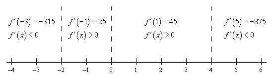
Make sure that you test your points in the derivative. One of the more common mistakes here is to test the points in the function instead! Recall that we know that the derivative will be the same sign in each region. The only place that the derivative can change signs is at the critical points and we’ve marked the only critical points on the number line.
So, it looks like we’ve got the following intervals of increase and decrease.
\[\begin{align*}{\mbox{Increase :}} & - 2 < x < 0{\mbox{ and }}0 < x < 4\\ {\mbox{Decrease : }} & - \infty < x < - 2{\mbox{ and }}4 < x < \infty \end{align*}\]In this example we used the fact that the only place that a derivative can change sign is at the critical points. Also, the critical points for this function were those for which the derivative was zero. However, the same thing can be said for critical points where the derivative doesn’t exist. This is nice to know. A function, in this section a derivative, can change signs where it is zero or doesn’t exist. In the previous chapter all our examples of this type had only critical points where the derivative was zero. Now, that we know more about critical points we’ll also see an example or two later on with critical points where the derivative doesn’t exist.
If you aren’t sure you believe that functions (they don’t have to be derivatives of course) can change sign where they don’t exist consider \(f\left( x \right) = \frac{1}{x}\) . This function clearly does not exist at \(x = 0\) and is negative if \(x < 0\) and positive if \(x > 0\) and so does change sign at the point where it does not exist. Be careful to not assume this will always be true however. Take \(f\left( x \right) = \frac{1}{{{x^2}}}\) for example. Again, this clearly does not exist at \(x = 0\) and yet is positive on both sides of \(x = 0\).
So, just to reiterate one more time. Functions, regardless of whether they are derivatives or not, may (but are not guaranteed to) change sign where they are either zero or do not exist.
Now that we have the previous “reminder” example out of the way let’s move into some new material. Once we have the intervals of increasing and decreasing for a function we can use this information to get a sketch of the graph. Note that the sketch, at this point, may not be super accurate when it comes to the curvature of the graph, but it will at least have the basic shape correct. To get the curvature of the graph correct we’ll need the information from the next section.
Let’s attempt to get a sketch of the graph of the function we used in the previous example.
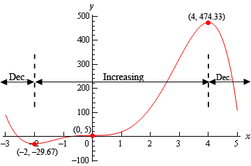
There really isn’t a whole lot to this example. Whenever we sketch a graph it’s nice to have a few points on the graph to give us a starting place. So we’ll start by the function at the critical points. These will give us some starting points when we go to sketch the graph. These points are,
\[f\left( { - 2} \right) = - \frac{89}{3} = - 29.67\hspace{0.25in}f\left( 0 \right) = 5\hspace{0.5in}f\left( 4 \right) = \frac{1423}{3} = 474.33\]Once these points are graphed we go to the increasing and decreasing information and start sketching. For reference purposes here is the increasing/decreasing information.
\[\begin{align*}{\mbox{Increase :}} & - 2 < x < 0{\mbox{ and }}0 < x < 4\\ {\mbox{Decrease : }} & - \infty < x < - 2{\mbox{ and }}4 < x < \infty \end{align*}\]Note that we are only after a sketch of the graph. As noted before we started this example we won’t be able to accurately predict the curvature of the graph at this point. However, even without this information we will still be able to get a basic idea of what the graph should look like.
To get this sketch we start at the very left of the graph and knowing that the graph must be decreasing and will continue to decrease until we get to \(x = - 2\). At this point the function will continue to increase until it gets to \(x = 4\). However, note that during the increasing phase it does need to go through the point at \(x = 0\) and at this point we also know that the derivative is zero here and so the graph goes through \(x = 0\)horizontally. Finally, once we hit \(x = 4\) the graph starts, and continues, to decrease. Also, note that just like at \(x = 0\) the graph will need to be horizontal when it goes through the other two critical points as well.
Here is the graph of the function. We, of course, used a graphical program to generate this graph, however, outside of some potential curvature issues if you followed the increasing/decreasing information and had all the critical points plotted first you should have something similar to this.
Let’s use the sketch from this example to give us a very nice test for classifying critical points as relative maximums, relative minimums or neither minimums or maximums.
Recall from the Minimum and Maximum Values section that all relative extrema of a function come from the list of critical points. The graph in the previous example has two relative extrema and both occur at critical points as the we predicted in that section. Note as well that we’ve got a critical point that isn’t a relative extrema (\(x = 0\)). This is okay since there is no reason to think that all critical points will be relative extrema. We only know that relative extrema will come from the list of critical points.
In the sketch of the graph from the previous example we can see that to the left of \(x = - 2\) the graph is decreasing and to the right of \(x = - 2\) the graph is increasing and \(x = - 2\) is a relative minimum. In other words, the graph is behaving around the minimum exactly as it would have to be in order for \(x = - 2\) to be a minimum. The same thing can be said for the relative maximum at \(x = 4\). The graph is increasing on the left and decreasing on the right exactly as it must be in order for \(x = 4\) to be a maximum. Finally, the graph is increasing on both sides of \(x = 0\) and so this critical point can’t be a minimum or a maximum.
These ideas can be generalized to arrive at a nice way to test if a critical point is a relative minimum, relative maximum or neither. If \(x = c\) is a critical point and the function is decreasing to the left of \(x = c\) and is increasing to the right then \(x = c\) must be a relative minimum of the function. Likewise, if the function is increasing to the left of \(x = c\) and decreasing to the right then \(x = c\) must be a relative maximum of the function. Finally, if the function is increasing on both sides of \(x = c\) or decreasing on both sides of \(x = c\) then \(x = c\) can be neither a relative minimum nor a relative maximum.
These ideas can be summarized up in the following test.
First Derivative Test
Suppose that \(x = c\) is a critical point of \(f\left( x \right)\) then,
- If \(f'\left( x \right) > 0\) to the left of \(x = c\) and \(f'\left( x \right) < 0\) to the right of \(x = c\) then \(x = c\) is a relative maximum.
- If \(f'\left( x \right) < 0\) to the left of \(x = c\) and \(f'\left( x \right) > 0\) to the right of \(x = c\) then \(x = c\) is a relative minimum.
- If \(f'\left( x \right)\) is the same sign on both sides of \(x = c\) then \(x = c\) is neither a relative maximum nor a relative minimum.
It is important to note here that the first derivative test will only classify critical points as relative extrema and not as absolute extrema. As we recall from the Finding Absolute Extrema section absolute extrema are largest and smallest function values and may not even exist or be critical points if they do exist.
The first derivative test is exactly that, a test using the first derivative. It doesn’t ever use the value of the function and so no conclusions can be drawn from the test about the relative “size” of the function at the critical points (which would be needed to identify absolute extrema) and can’t even begin to address the fact that absolute extrema may not occur at critical points.
Let’s take at another example.
First, we’ll need the derivative so we can get our hands on the critical points. Note as well that we’ll do some simplification on the derivative to help us find the critical points.
\[\begin{align*}g'\left( t \right) & = {\left( {{t^2} - 4} \right)^{\frac{1}{3}}} + \frac{2}{3}{t^2}{\left( {{t^2} - 4} \right)^{ - \frac{2}{3}}}\\ & = {\left( {{t^2} - 4} \right)^{\frac{1}{3}}} + \frac{{2{t^2}}}{{3{{\left( {{t^2} - 4} \right)}^{\frac{2}{3}}}}}\\ & = \frac{{3\left( {{t^2} - 4} \right) + 2{t^2}}}{{3{{\left( {{t^2} - 4} \right)}^{\frac{2}{3}}}}}\\ & = \frac{{5{t^2} - 12}}{{3{{\left( {{t^2} - 4} \right)}^{\frac{2}{3}}}}}\end{align*}\]So, it looks like we’ll have four critical points here. They are,
\[\begin{align*}t & = \pm \,2 & \hspace{1.0in} & {\mbox{The derivative doesn't exist here}}{\mbox{.}}\\ t & = \pm \sqrt {\frac{{12}}{5}} = \pm 1.549 & \hspace{1.0in} & {\mbox{The derivative is zero here}}{\mbox{.}}\end{align*}\]Finding the intervals of increasing and decreasing will also give the classification of the critical points so let’s get those first. Here is a number line with the critical points graphed and test points.
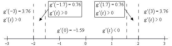
So, it looks like we’ve got the following intervals of increasing and decreasing.
\[\begin{align*}{\mbox{Increase :}} & - \infty < x < - 2,\,\,\, - 2 < x < - \sqrt {\frac{{12}}{5}} ,\,\,\,\sqrt {\frac{12}{5}} < x < 2,\,\,\,\,\& \,\,\,2 < x < \infty \\ {\mbox{Decrease : }} & - \sqrt {\frac{{12}}{5}} < x < \sqrt {\frac{{12}}{5}} \end{align*}\]From this it looks like \(t = - 2\) and \(t = 2\) are neither relative minimum or relative maximums since the function is increasing on both side of them. On the other hand, \(t = - \sqrt {\frac{12}{5}} \) is a relative maximum and \(t = \sqrt {\frac{12}{5}} \)is a relative minimum.
For completeness sake here is the graph of the function. Note that this graph is a little trickier to sketch based only on the increasing and decreasing information. It is only presented here for reference so you can see what it looks like.
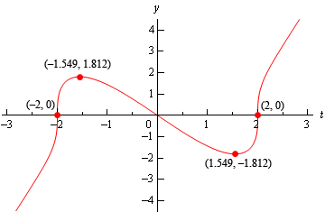
In the previous example the two critical points where the derivative didn’t exist ended up not being relative extrema. Do not read anything into this. They often will be relative extrema. Check out Example 5 in the Absolute Extrema to see an example of one such critical point.
Let’s work a couple more examples.
where \(x\) is in miles. Assume that if \(x\) is positive we are to the east of the initial point of measurement and if \(x\) is negative we are to the west of the initial point of measurement.
If we start 25 miles to the west of the initial point of measurement and drive until we are 25 miles east of the initial point how many miles of our drive were we driving up an incline?
Okay, this is just a really fancy way of asking what the intervals of increasing and decreasing are for the function on the interval \(\left[ { - 25,25} \right]\). So, we first need the derivative of the function.
\[E'\left( x \right) = - \frac{1}{4}\sin \left( {\frac{x}{4}} \right) + \frac{{\sqrt 3 }}{4}\cos \left( {\frac{x}{4}} \right)\]Setting this equal to zero gives,
\[\begin{align*} - \frac{1}{4}\sin \left( {\frac{x}{4}} \right) + \frac{{\sqrt 3 }}{4}\cos \left( {\frac{x}{4}} \right) & = 0\\ \tan \left( {\frac{x}{4}} \right) & = \sqrt 3 \end{align*}\]The solutions to this and hence the critical points are,
\[\begin{array}{*{20}{c}}{\displaystyle \frac{x}{4} = 1.0472 + 2\pi n,\,\,n = 0, \pm 1, \pm 2, \ldots }\\{\displaystyle \frac{x}{4} = 4.1888 + 2\pi n,\,\,n = 0, \pm 1, \pm 2, \ldots }\end{array}\hspace{0.25in} \Rightarrow \hspace{0.25in}\begin{array}{*{20}{c}}{x = 4.1888 + 8\pi n,\,\,n = 0, \pm 1, \pm 2, \ldots \,\,}\\{x = 16.7552 + 8\pi n,\,\,n = 0, \pm 1, \pm 2, \ldots }\end{array}\]I’ll leave it to you to check that the critical points that fall in the interval that we’re after are,
\[ - 20.9439,\,\,\, - 8.3775,\,\,\,4.1888,\,\,\,16.7552\]Here is the number line with the critical points and test points.
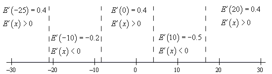
So, it looks like the intervals of increasing and decreasing are,
\[\begin{align*}{\mbox{Increase :}} & - 25 < x < - 20.9439, \,\,\, - 8.3775 < x < 4.1888{\mbox{ and }} 16.7552 < x < 25\\ {\mbox{Decrease : }} & - 20.9439 < x < - 8.3775{\mbox{ and }} 4.1888 < x < 16.7552 \end{align*}\]Notice that we had to end our intervals at -25 and 25 since we’ve done no work outside of these points and so we can’t really say anything about the function outside of the interval \(\left[ { - 25,25} \right]\).
From the intervals we can actually answer the question. We were driving on an incline during the intervals of increasing and so the total number of miles is,
\[\begin{align*}{\mbox{Distance }} & = \left( { - 20.9439 - \left( { - 25} \right)} \right) + \left( {4.1888 - \left( { - 8.3775} \right)} \right) + \left( {25 - 16.7552} \right)\\ & = 24.8652{\mbox{ miles}}\end{align*}\]Even though the problem didn’t ask for it we can also classify the critical points that are in the interval \(\left[ { - 25,25} \right]\).
\[\begin{align*}{\mbox{Relative Maximums : }} & - 20.9439,4.1888\\ {\mbox{Relative Minimums : }} & - 8.3775,16.7552\end{align*}\]Determine if the population ever decreases in the first two years.
So, again we are really after the intervals and increasing and decreasing in the interval [0,2].
We found the only critical point to this function back in the Critical Points section to be,
\[x = \frac{1}{{3\sqrt {\bf{e}} }} = 0.202\]Here is a number line for the intervals of increasing and decreasing.
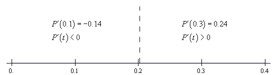
So, it looks like the population will decrease for a short period and then continue to increase forever.
Also, while the problem didn’t ask for it we can see that the single critical point is a relative minimum.
In this section we’ve seen how we can use the first derivative of a function to give us some information about the shape of a graph and how we can use this information in some applications.
Using the first derivative to give us information about a whether a function is increasing or decreasing is a very important application of derivatives and arises on a fairly regular basis in many areas.