Section 2.4 : Bernoulli Differential Equations
In this section we are going to take a look at differential equations in the form,
\[y' + p\left( x \right)y = q\left( x \right){y^n}\]where \(p(x)\) and \(q(x)\) are continuous functions on the interval we’re working on and \(n\) is a real number. Differential equations in this form are called Bernoulli Equations.
First notice that if \(n = 0\) or \(n = 1\) then the equation is linear and we already know how to solve it in these cases. Therefore, in this section we’re going to be looking at solutions for values of \(n\) other than these two.
In order to solve these we’ll first divide the differential equation by \({y^n}\) to get,
\[{y^{ - n}}\,y' + p\left( x \right){y^{1 - n}} = q\left( x \right)\]We are now going to use the substitution \(v = {y^{1 - n}}\) to convert this into a differential equation in terms of \(v\). As we’ll see this will lead to a differential equation that we can solve.
We are going to have to be careful with this however when it comes to dealing with the derivative, \(y'\). We need to determine just what \(y'\) is in terms of our substitution. This is easier to do than it might at first look to be. All that we need to do is differentiate both sides of our substitution with respect to \(x\). Remember that both \(v\) and \(y\) are functions of \(x\) and so we’ll need to use the chain rule on the right side. If you remember your Calculus I you’ll recall this is just implicit differentiation. So, taking the derivative gives us,
\[v' = \left( {1 - n} \right){y^{ - n}}y'\]Now, plugging this as well as our substitution into the differential equation gives,
\[\frac{1}{{1 - n}}v' + p\left( x \right)v = q\left( x \right)\]This is a linear differential equation that we can solve for \(v\) and once we have this in hand we can also get the solution to the original differential equation by plugging \(v\) back into our substitution and solving for \(y\).
Let’s take a look at an example.
So, the first thing that we need to do is get this into the “proper” form and that means dividing everything by \({y^2}\). Doing this gives,
\[{y^{ - 2}}\,y' + \frac{4}{x}{y^{ - 1}} = {x^3}\]The substitution and derivative that we’ll need here is,
\[v = {y^{ - 1}}\hspace{0.25in}v' = - {y^{ - 2}}y'\]With this substitution the differential equation becomes,
\[ - v' + \frac{4}{x}v = {x^3}\]So, as noted above this is a linear differential equation that we know how to solve. We’ll do the details on this one and then for the rest of the examples in this section we’ll leave the details for you to fill in. If you need a refresher on solving linear differential equations then go back to that section for a quick review.
Here’s the solution to this differential equation.
\[v' - \frac{4}{x}v = - {x^3}\hspace{0.25in}\,\,\,\, \Rightarrow \hspace{0.25in}\mu \left( x \right) = {{\bf{e}}^{\int{{ - \,\,\frac{4}{x}\,dx}}}} = {{\bf{e}}^{ - 4\,\,\ln \left| x \right|}} = {x^{ - 4}}\] \[\begin{align*}\int{{{{\left( {{x^{ - 4}}v} \right)}^\prime }\,dx}} & = \int{{ - {x^{ - 1}}\,dx}}\\ {x^{ - 4}}v & = - \ln \left| x \right| + c\hspace{0.25in} \Rightarrow \hspace{0.25in}v\left( x \right) = c{x^4} - {x^4}\ln x\end{align*}\]Note that we dropped the absolute value bars on the \(x\) in the logarithm because of the assumption that \(x > 0\).
Now we need to determine the constant of integration. This can be done in one of two ways. We can convert the solution above into a solution in terms of \(y\) and then use the original initial condition or we can convert the initial condition to an initial condition in terms of \(v\) and use that. Because we’ll need to convert the solution to \(y\)’s eventually anyway and it won’t add that much work in we’ll do it that way.
So, to get the solution in terms of \(y\) all we need to do is plug the substitution back in. Doing this gives,
\[{y^{ - 1}} = {x^4}\left( {c - \ln x} \right)\]At this point we can solve for \(y\) and then apply the initial condition or apply the initial condition and then solve for \(y\). We’ll generally do this with the later approach so let’s apply the initial condition to get,
\[{\left( { - 1} \right)^{ - 1}} = c{2^4} - {2^4}\ln 2\hspace{0.25in} \Rightarrow \hspace{0.25in}c = \ln 2 - \frac{1}{{16}}\]Plugging in for \(c\) and solving for \(y\) gives,
\[y\left( x \right) = \frac{1}{{{x^4}\left( {\ln 2 - \frac{1}{{16}} - \ln x} \right)}} = \frac{{ - 16}}{{{x^4}\left( {1 + 16\ln x - 16\ln 2} \right)}} = \frac{{ - 16}}{{{x^4}\left( {1 + 16\ln \frac{x}{2}} \right)}}\]Note that we did a little simplification in the solution. This will help with finding the interval of validity.
Before finding the interval of validity however, we mentioned above that we could convert the original initial condition into an initial condition for \(v\). Let’s briefly talk about how to do that. To do that all we need to do is plug \(x = 2\) into the substitution and then use the original initial condition. Doing this gives,
\[v\left( 2 \right) = {y^{ - 1}}\left( 2 \right) = {\left( { - 1} \right)^{ - 1}} = - 1\]So, in this case we got the same value for \(v\) that we had for \(y\). Don’t expect that to happen in general if you chose to do the problems in this manner.
Okay, let’s now find the interval of validity for the solution. First, we already know that \(x > 0\) and that means we’ll avoid the problems of having logarithms of negative numbers and division by zero at \(x = 0\). So, all that we need to worry about then is division by zero in the second term and this will happen where,
\[\begin{align*}1 + 16\ln \frac{x}{2} & = 0\\ \ln \frac{x}{2} & = - \frac{1}{{16}}\\ \frac{x}{2} & = {{\bf{e}}^{ - \,\frac{1}{{16}}}}\hspace{0.25in} \Rightarrow \hspace{0.25in}x = 2{{\bf{e}}^{ - \,\frac{1}{{16}}}} \approx 1.8788\end{align*}\]The two possible intervals of validity are then,
\[0 < x < 2{{\bf{e}}^{ - \,\frac{1}{{16}}}}\hspace{0.25in}2{{\bf{e}}^{ - \,\frac{1}{{16}}}} < x < \infty \]and since the second one contains the initial condition we know that the interval of validity is then \(2{{\bf{e}}^{ - \,\frac{1}{{16}}}} < x < \infty \).
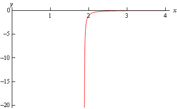
Here is a graph of the solution.

Let’s do a couple more examples and as noted above we’re going to leave it to you to solve the linear differential equation when we get to that stage.
The first thing we’ll need to do here is multiply through by \({y^2}\) and we’ll also do a little rearranging to get things into the form we’ll need for the linear differential equation. This gives,
\[{y^2}\,y' - 5{y^3} = {{\bf{e}}^{ - 2\,x}}\]The substitution here and its derivative is,
\[v = {y^3}\hspace{0.25in}v' = 3{y^2}y'\]Plugging the substitution into the differential equation gives,
\[\frac{1}{3}v' - 5v = {{\bf{e}}^{ - 2\,x}}\hspace{0.25in} \Rightarrow \hspace{0.25in}v' - 15v = 3{{\bf{e}}^{ - 2\,x}}\hspace{0.25in}\mu \left( x \right) = {{\bf{e}}^{ - 15\,x}}\]We rearranged a little and gave the integrating factor for the linear differential equation solution. Upon solving we get,
\[v\left( x \right) = c{{\bf{e}}^{15\,x}} - \frac{3}{{17}}{{\bf{e}}^{ - 2\,x}}\]Now go back to \(y\)’s.
\[{y^3} = c{{\bf{e}}^{15\,x}} - \frac{3}{{17}}{{\bf{e}}^{ - 2\,x}}\]Applying the initial condition and solving for \(c\) gives,
\[8 = c - \frac{3}{{17}}\hspace{0.25in} \Rightarrow \hspace{0.25in}c = \frac{{139}}{{17}}\]Plugging in \(c\) and solving for \(y\) gives,
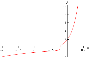
\[y\left( x \right) = {\left( {\frac{{139{{\bf{e}}^{15\,x}} - 3{{\bf{e}}^{ - 2\,x}}}}{{17}}} \right)^{\frac{1}{3}}}\]There are no problem values of \(x\) for this solution and so the interval of validity is all real numbers. Here’s a graph of the solution.

First get the differential equation in the proper form and then write down the substitution.
\[6{y^{ - 4}}y' - 2{y^{ - 3}} = x\hspace{0.25in} \Rightarrow \hspace{0.25in}v = {y^{ - 3}}\hspace{0.25in}v' = - 3{y^{ - 4}}y'\]Plugging the substitution into the differential equation gives,
\[ - 2v' - 2v = x\hspace{0.25in} \Rightarrow \hspace{0.25in}\,\,v' + v = - \frac{1}{2}x\hspace{0.25in}\mu \left( x \right) = {{\bf{e}}^{\,x}}\]Again, we’ve rearranged a little and given the integrating factor needed to solve the linear differential equation. Upon solving the linear differential equation we have,
\[v\left( x \right) = - \frac{1}{2}\left( {x - 1} \right) + c{{\bf{e}}^{ - \,x}}\]Now back substitute to get back into \(y\)’s.
\[{y^{ - 3}} = - \frac{1}{2}\left( {x - 1} \right) + c{{\bf{e}}^{ - \,x}}\]Now we need to apply the initial condition and solve for \(c\).
\[ - \frac{1}{8} = \frac{1}{2} + c\hspace{0.25in} \Rightarrow \hspace{0.25in}c = - \frac{5}{8}\]Plugging in \(c\) and solving for \(y\) gives,
\[y\left( x \right) = - \frac{2}{{{{\left( {4x - 4 + 5{{\bf{e}}^{ - \,x}}} \right)}^{\frac{1}{3}}}}}\]Next, we need to think about the interval of validity. In this case all we need to worry about it is division by zero issues and using some form of computational aid (such as Maple or Mathematica) we will see that the denominator of our solution is never zero and so this solution will be valid for all real numbers.
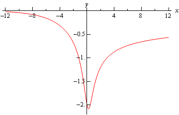
Here is a graph of the solution.

To this point we’ve only worked examples in which n was an integer (positive and negative) and so we should work a quick example where n is not an integer.
Let’s first get the differential equation into proper form.
\[y' + \frac{1}{x}y = {y^{\frac{1}{2}}}\hspace{0.25in} \Rightarrow \hspace{0.25in}{y^{ - \,\frac{1}{2}}}y' + \frac{1}{x}{y^{\frac{1}{2}}} = 1\]The substitution is then,
\[v = {y^{\frac{1}{2}}}\hspace{0.25in}v' = \frac{1}{2}{y^{ - \,\frac{1}{2}}}y'\]Now plug the substitution into the differential equation to get,
\[2v' + \frac{1}{x}v = 1\hspace{0.25in} \Rightarrow \hspace{0.25in}\,\,\,\,\,\,\,\,\,v' + \frac{1}{{2x}}v = \frac{1}{2}\hspace{0.25in}\mu \left( x \right) = {x^{\frac{1}{2}}}\]As we’ve done with the previous examples we’ve done some rearranging and given the integrating factor needed for solving the linear differential equation. Solving this gives us,
\[v\left( x \right) = \frac{1}{3}x + c{x^{ - \,\frac{1}{2}}}\]In terms of \(y\) this is,
\[{y^{\frac{1}{2}}} = \frac{1}{3}x + c{x^{ - \,\frac{1}{2}}}\]Applying the initial condition and solving for \(c\) gives,
\[0 = \frac{1}{3} + c\hspace{0.25in} \Rightarrow \hspace{0.25in}c = - \frac{1}{3}\]Plugging in for \(c\) and solving for \(y\) gives us the solution.
\[y\left( x \right) = {\left( {\frac{1}{3}x - \frac{1}{3}{x^{ - \,\frac{1}{2}}}} \right)^2} = \frac{{{x^3} - 2{x^{\frac{3}{2}}} + 1}}{{9x}}\]Note that we multiplied everything out and converted all the negative exponents to positive exponents to make the interval of validity clear here. Because of the root (in the second term in the numerator) and the \(x\) in the denominator we can see that we need to require \(x > 0\) in order for the solution to exist and it will exist for all positive \(x\)’s and so this is also the interval of validity.
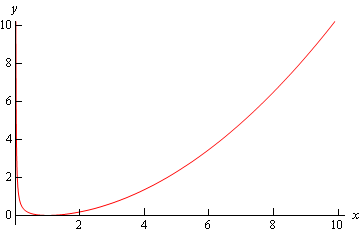
Here is the graph of the solution.
