Differential Equations

Show Mobile Notice Show All Notes Hide All Notes

Mobile Notice

You appear to be on a device with a "narrow" screen width (i.e. you are probably on a mobile phone). Due to the nature of the mathematics on this site it is best viewed in landscape mode. If your device is not in landscape mode many of the equations will run off the side of your device (you should be able to scroll/swipe to see them) and some of the menu items will be cut off due to the narrow screen width.

Section 5.12 : Modeling

In this section we’re going to go back and revisit the idea of modeling only this time we’re going to look at it in light of the fact that we now know how to solve systems of differential equations.

We’re not actually going to be solving any differential equations in this section. Instead we’ll just be setting up a couple of problems that are extensions of some of the work that we’ve done in earlier modeling sections whether it is the first order modeling or the vibrations work we did in the second order chapter. Almost all of the systems that we’ll be setting up here will be nonhomogeneous systems (which we only briefly looked at), will be nonlinear (which we didn’t look at) and/or will involve systems with more than two differential equations (which we didn’t look at, although most of what we do know will still be true).

Mixing Problems

Let’s start things by looking at a mixing problem. The last time we saw these was back in the first order chapter. In those problems we had a tank of liquid with some type of contaminate dissolved in it. Liquid, possibly with more contaminate dissolved in it, entered the tank and liquid left the tank. In this situation we want to extend things out to the following situation.

This is a sketch of two tanks filled with some liquid. The tank on the left is labeled “Tank 1” and the tank on the right is labeled “Tank 2”. Above each tank is a pipe with an arrow pointing downwards indicating liquid is flowing out of the pipe and into the tank below it. Near the top of each tank there is a pipe connecting them with an arrow pointing to the left indicating liquid is flowing from Tank 2 into Tank 1. Below this is another pipe connecting the two tanks. In the middle of this pipe there is a “T” connection with a pipe dropping vertically out of the “T” and the pipe coming out of the “T” to the right is smaller in radius than the pipe to the left of the “T”. There are arrows indicating that liquid is flowing out of Tank 1 into Tank 2 with a portion of the liquid flowing out of the system via the vertical pipe coming out of the “T” connection.

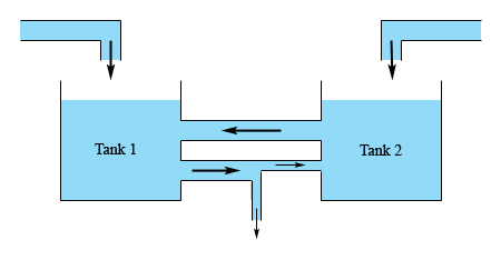
We’ll now have two tanks that are interconnected with liquid potentially entering both and with an exit for some of the liquid if we need it (as illustrated by the lower connection). For this situation we’re going to make the following assumptions.

The inflow and outflow from each tank are equal, or in other words the volume in each tank is constant. When we worked with a single tank we didn’t need to worry about this, but here if we don’t well end up with a system with nonconstant coefficients and those can be quite difficult to solve.
The concentration of the contaminate in each tank is the same at each point in the tank. In reality we know that this won’t be true but without this assumption we’d need to deal with partial differential equations.
The concentration of contaminate in the outflow from tank 1 (the lower connection in the figure above) is the same as the concentration in tank 1. Likewise, the concentration of contaminate in the outflow from tank 2 (the upper connection) is the same as the concentration in tank 2.
The outflow from tank 1 is split and only some of the liquid exiting tank 1 actually reaches tank 2. The remainder exits the system completely. Note that if we don’t want any liquid to completely exit the system we can think of the exit as having a value that is turned off. Also note that we could just as easily done the same thing for the outflow from tank 2 if we’d wanted to.

Let’s take a look at a quick example.

Example 1 Two 1000 liter tanks are with salt water. Tank 1 contains 800 liters of water initially containing 20 grams of salt dissolved in it and tank 2 contains 1000 liters of water and initially has 80 grams of salt dissolved in it. Salt water with a concentration of ½ gram/liter of salt enters tank 1 at a rate of 4 liters/hour. Fresh water enters tank 2 at a rate of 7 liters/hour. Through a connecting pipe water flows from tank 2 into tank 1 at a rate of 10 liters/hour. Through a different connecting pipe 14 liters/hour flows out of tank 1 and 11 liters/hour are drained out of the pipe (and hence out of the system completely) and only 3 liters/hour flows back into tank 2. Set up the system that will give the amount of salt in each tank at any given time.

Show Solution

Okay, let ${Q_1}\left( t \right)$ and ${Q_2}\left( t \right)$ be the amount of salt in tank 1 and tank 2 at any time $t$ respectively. Now all we need to do is set up a differential equation for each tank just as we did back when we had a single tank. The only difference is that we now need to deal with the fact that we’ve got a second inflow to each tank and the concentration of the second inflow will be the concentration of the other tank.

Recall that the basic differential equation is the rate of change of salt ($Q'$) equals the rate at which salt enters minus the rate at salt leaves. Each entering/leaving rate is found by multiplying the flow rate times the concentration.

Here is the differential equation for tank 1.

\[\begin{align*}{{Q'}_1} & = \left( 4 \right)\left( {\frac{1}{2}} \right) + \left( {10} \right)\left( {\frac{{{Q_2}}}{{1000}}} \right) - \left( {14} \right)\left( {\frac{{{Q_1}}}{{800}}} \right)\hspace{0.25in}{Q_1}\left( 0 \right) = 20\\ & = 2 + \frac{{{Q_2}}}{{100}} - \frac{{7{Q_1}}}{{400}}\end{align*}\]

In this differential equation the first pair of numbers is the salt entering from the external inflow. The second set of numbers is the salt that entering into the tank from the water flowing in from tank 2. The third set is the salt leaving tank as water flows out.

Here’s the second differential equation.

\[\begin{align*}{{Q'}_2} & = \left( 7 \right)\left( 0 \right) + \left( 3 \right)\left( {\frac{{{Q_1}}}{{800}}} \right) - \left( {10} \right)\left( {\frac{{{Q_2}}}{{1000}}} \right)\hspace{0.25in}{Q_2}\left( 0 \right) = 80\\ & = \frac{{3{Q_1}}}{{800}} - \frac{{{Q_2}}}{{100}}\end{align*}\]

Note that because the external inflow into tank 2 is fresh water the concentration of salt in this is zero.

In summary here is the system we’d need to solve,

\[\begin{align*}{{Q'}_1} & = 2 + \frac{{{Q_2}}}{{100}} - \frac{{7{Q_1}}}{{400}}\hspace{0.25in}{Q_1}\left( 0 \right) = 20\\ {{Q'}_2} & = \frac{{3{Q_1}}}{{800}} - \frac{{{Q_2}}}{{100}}\hspace{0.25in}{Q_2}\left( 0 \right) = 80\end{align*}\]

This is a nonhomogeneous system because of the first term in the first differential equation. If we had fresh water flowing into both of these we would in fact have a homogeneous system.

Population

The next type of problem to look at is the population problem. Back in the first order modeling section we looked at some population problems. In those problems we looked at a single population and often included some form of predation. The problem in that section was we assumed that the amount of predation would be constant. This however clearly won’t be the case in most situations. The amount of predation will depend upon the population of the predators and the population of the predators will depend, as least partially, upon the population of the prey.

So, in order to more accurately (well at least more accurate than what we originally did) we really need to set up a model that will cover both populations, both the predator and the prey. These types of problems are usually called predator-prey problems. Here are the assumptions that we’ll make when we build up this model.

The prey will grow at a rate that is proportional to its current population if there are no predators.
The population of predators will decrease at a rate proportional to its current population if there is no prey.
The number of encounters between predator and prey will be proportional to the product of the populations.
Each encounter between the predator and prey will increase the population of the predator and decrease the population of the prey.

So, given these assumptions let’s write down the system for this case.

Example 2 Write down the system of differential equations for the population of predators and prey using the assumptions above.

Show Solution

We’ll start off by letting $x$ represent the population of the predators and $y$ represent the population of the prey.

Now, the first assumption tells us that, in the absence of predators, the prey will grow at a rate of $ay$ where $a > 0$. Likewise, the second assumption tells us that, in the absence of prey, the predators will decrease at a rate of $ - bx$ where $b > 0$.

Next, the third and fourth assumptions tell us how the population is affected by encounters between predators and prey. So, with each encounter the population of the predators will increase at a rate of $\alpha xy$ and the population of the prey will decrease at a rate of $ - \beta xy$ where $\alpha > 0$ and $\beta > 0$.

Putting all of this together we arrive at the following system.

\[\begin{align*}x' & = - bx + \alpha xy = x\left( {\alpha y - b} \right)\\ y' & = ay - \beta xy = y\left( {a - \beta x} \right)\end{align*}\]

Note that this is a nonlinear system and we’ve not (nor will we here) discuss how to solve this kind of system. We simply wanted to give a “better” model for some population problems and to point out that not all systems will be nice and simple linear systems.

Mechanical Vibrations

When we first looked at mechanical vibrations we looked at a single mass hanging on a spring with the possibility of both a damper and/or an external force acting on the mass. Here we want to look at the following situation.

$This is a sketch of a horizontal surface with two vertical surfaces coming directly up out of the right and left ends. Spaced at approximately 1/3 and 2/3 distance from the left vertical surface are objects. The right object is labeled $m_{2}$ and has a vertical line dropping out of the bottom of it labeled $x_{2}=0$. This vertical line has an arrow pointing right labeled “+ Displacement”. The left object is labeled $m_{1}$ and has a vertical line dropping out of the bottom of it labeled $x_{1}=0$. This vertical line has an arrow pointing right labeled “+ Displ.”. There is a spring connecting the left vertical surface and the left object labeled $k_{1}$. There is a spring connecting the two objects labeled $k_{2}$. There is a spring connecting the right object and the right vertical surface labeled $k_{3}$.$

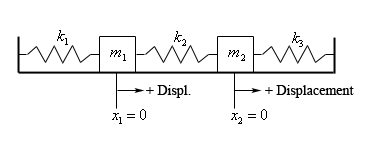
In the figure above we are assuming that the system is at rest. In other words, all three springs are currently at their natural lengths and are not exerting any forces on either of the two masses and that there are no currently any external forces acting on either mass.

We will use the following assumptions about this situation once we start the system in motion.

${x_1}$ will measure the displacement of mass ${m_1}$ from its equilibrium (i.e. resting) position and ${x_2}$ will measure the displacement of mass ${m_2}$ from its equilibrium position.
As noted in the figure above all displacement will be assumed to be positive if it is to the right of equilibrium position and negative if to the left of the equilibrium position.
All forces acting to the right are positive forces and all forces acting to the left are negative forces.
The spring constants, ${k_1}$, ${k_2}$, and ${k_3}$, are all positive and may or may not be the same value.
The surface that the system is sitting on is frictionless and so the mass of each of the objects will not affect the system in any way.

Before writing down the system for this case recall that the force exerted by the spring on each mass is the spring constant times the amount that the spring has been compressed or stretched and we’ll need to be careful with signs to make sure that the force is acting in the correct direction.

Example 3 Write down the system of differential equations for the spring and mass system above.

Show Solution

To help us out let’s first take a quick look at a situation in which both of the masses have been moved. This is shown below.

$This is a sketch of a horizontal surface with two vertical surfaces coming directly up out of the right and left ends. Spaced at approximately 1/3 and 2/3 distance from the left vertical surface are two vertical lines dropping out of the horizontal surface. The left vertical line is labeled $x{1}=0$ and to the right of this is an object labeled $m_{1}$ and out of the bottom of this object a dashed line drops straight down. The distance between the dashed line and the left vertical line is shown as $x_{1}$. The right vertical line is labeled $x{s}=0$ and to the right of this is an object labeled $m_{s}$ and out of the bottom of this object a dashed line drops straight down. The distance between the dashed line and the right vertical line is shown as $x_{2}$. There is a spring connecting the left vertical surface and the left object labeled $k_{1}$. There is a spring connecting the two objects labeled $k_{2}$. There is a spring connecting the right object and the right vertical surface labeled $k_{3}$.$

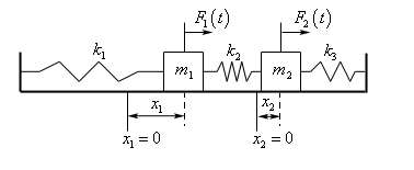
Before proceeding let’s note that this is only a representation of a typical case, but most definitely not all possible cases.

In this case we’re assuming that both ${x_1}$ and ${x_2}$ are positive and that ${x_2} - {x_1} < 0$, or in other words, both masses have been moved to the right of their respective equilibrium points and that ${m_1}$ has been moved farther than ${m_2}$. So, under these assumptions on ${x_1}$ and ${x_2}$ we know that the spring on the left (with spring constant ${k_1}$) has been stretched past it’s natural length while the middle spring (spring constant ${k_2}$) and the right spring (spring constant ${k_3}$) are both under compression.

Also, we’ve shown the external forces, ${F_1}\left( t \right)$ and ${F_2}\left( t \right)$, as present and acting in the positive direction. They do not, in practice, need to be present in every situation in which case we will assume that ${F_1}\left( t \right) = 0$ and/or ${F_2}\left( t \right) = 0$. Likewise, if the forces are in fact acting in the negative direction we will then assume that ${F_1}\left( t \right) < 0$ and/or ${F_2}\left( t \right) < 0$.

Before proceeding we need to talk a little bit about how the middle spring will behave as the masses move. Here are all the possibilities that we can have and the affect each will have on ${x_2} - {x_1}$. Note that in each case the amount of compression/stretch in the spring is given by $\left| {{x_2} - {x_1}} \right|$ although we won’t be using the absolute value bars when we set up the differential equations.

If both mass move the same amount in the same direction then the middle spring will not have changed length and we’ll have ${x_2} - {x_1} = 0$.
If both masses move in the positive direction then the sign of ${x_2} - {x_1}$ will tell us which has moved more. If ${m_1}$ moves more than ${m_2}$ then the spring will be in compression and ${x_2} - {x_1} < 0$. Likewise, if ${m_2}$ moves more than ${m_1}$ then the spring will have been stretched and ${x_2} - {x_1} > 0$.
If both masses move in the negative direction we’ll have pretty much the opposite behavior as #2. If ${m_1}$ moves more than ${m_2}$ then the spring will have been stretched and ${x_2} - {x_1} > 0$. Likewise, if ${m_2}$ moves more than ${m_1}$ then the spring will be in compression and ${x_2} - {x_1} < 0$.
If ${m_1}$ moves in the positive direction and ${m_2}$ moves in the negative direction then the spring will be in compression and ${x_2} - {x_1} < 0$.
Finally, if ${m_1}$ moves in the negative direction and ${m_2}$ moves in the positive direction then the spring will have been stretched and ${x_2} - {x_1} > 0$.

Now, we’ll use the figure above to help us develop the differential equations (the figure corresponds to case 2 above…) and then make sure that they will also hold for the other cases as well.

Let’s start off by getting the differential equation for the forces acting on ${m_1}$. Here is a quick sketch of the forces acting on ${m_1}$ for the figure above.

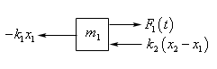
In this case ${x_1} > 0$ and so the first spring has been stretched and so will exert a negative (i.e. to the left) force on the mass. The force from the first spring is then$ - {k_1}{x_1}$ and the “-” is needed because the force is negative but both ${k_1}$ and ${x_1}$ are positive.

Next, because we’re assuming that ${m_1}$ has moved more than ${m_2}$ and both have moved in the positive direction we also know that ${x_2} - {x_1} < 0$. Because ${m_1}$ has moved more than ${m_2}$ we know that the second spring will be under compression and so the force should be acting in the negative direction on ${m_1}$ and so the force will be ${k_2}\left( {{x_2} - {x_1}} \right)$. Note that because ${k_2}$ is positive and ${x_2} - {x_1}$ is negative this force will have the correct sign (i.e. negative).

The differential equation for ${m_1}$ is then,

\[{m_1}{x''_1} = - \,{k_1}{x_1} + {k_2}\left( {{x_2} - {x_1}} \right) + {F_1}\left( t \right)\]

Note that this will also hold for all the other cases. If ${m_1}$ has been moved in the negative direction the force form the spring on the right that acts on the mass will be positive and $ - {k_1}{x_1}$ will be a positive quantity in this case. Next, if the middle mass has been stretched (i.e. ${x_2} - {x_1} > 0$) then the force from this spring on ${m_1}$ will be in the positive direction and ${k_2}\left( {{x_2} - {x_1}} \right)$ will be a positive quantity in this case. Therefore, this differential equation holds for all cases not just the one we illustrated at the start of this problem.

Let’s now write down the differential equation for all the forces that are acting on ${m_2}$. Here is a sketch of the forces acting on this mass for the situation sketched out in the figure above.

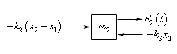
In this case ${x_2}$ is positive and so the spring on the right is under compression and will exert a negative force on ${m_2}$ and so this force should be $ - {k_3}{x_2}$, where the “-” is required because both ${k_3}$ and ${x_2}$ are positive. Also, the middle spring is still under compression but the force that it exerts on this mass is now a positive force, unlike in the case of ${m_1}$, and so is given by $ - {k_2}\left( {{x_2} - {x_1}} \right)$. The “-” on this force is required because ${x_2} - {x_1}$ is negative and the force must be positive.

The differential equation for ${m_2}$ is then,

\[{m_2}{x''_2} = - \,{k_3}{x_2} - {k_2}\left( {{x_2} - {x_1}} \right) + {F_2}\left( t \right)\]

We’ll leave it to you to verify that this differential equation does in fact hold for all the other cases.

Putting all of this together and doing a little rewriting will then give the following system of differential equations for this situation.

\[\begin{align*}{m_1}{{x''}_1} & = - \left( {{k_1} + \,{k_2}} \right){x_1} + {k_2}{x_2} + {F_1}\left( t \right)\\ {m_2}{{x''}_2} & = {k_2}{x_1} - \left( {{k_2} + \,{k_3}} \right){x_2} + {F_2}\left( t \right)\end{align*}\]

This is a system to two linear second order differential equations that may or may not be nonhomogeneous depending whether there are any external forces, ${F_1}\left( t \right)$ and ${F_2}\left( t \right)$, acting on the masses.

We have not talked about how to solve systems of second order differential equations. However, it can be converted to a system of first order differential equations as the next example shows and in many cases we could solve that.

Example 4 Convert the system from the previous example to a system of 1^st order differential equations.

Show Solution

This isn’t too hard to do. Recall that we did this for single higher order differential equations earlier in the chapter when we first started to look at systems. To convert this to a system of first order differential equations we can make the following definitions.

\[{u_1} = {x_1}\hspace{0.25in}{u_2} = {x'_1}\hspace{0.25in}{u_3} = {x_2}\hspace{0.25in}{u_4} = {x'_2}\]

We can then convert each of the differential equations as we did earlier in the chapter.

\[\begin{align*}{{u'}_1} & = {{x'}_1} = {u_2}\\ {{u'}_2} & = {{x''}_1} = \frac{1}{{{m_1}}}\left( { - \left( {{k_1} + \,{k_2}} \right){x_1} + {k_2}{x_2} + {F_1}\left( t \right)} \right) = \frac{1}{{{m_1}}}\left( { - \left( {{k_1} + \,{k_2}} \right){u_1} + {k_2}{u_3} + {F_1}\left( t \right)} \right)\\ {{u'}_3} & = {{x'}_2} = {u_4}\\ {{u'}_4} & = {{x''}_2} = \frac{1}{{{m_2}}}\left( {{k_2}{x_1} - \left( {{k_2} + \,{k_3}} \right){x_2} + {F_2}\left( t \right)} \right) = \frac{1}{{{m_2}}}\left( {{k_2}{u_1} - \left( {{k_2} + \,{k_3}} \right){u_3} + {F_2}\left( t \right)} \right)\end{align*}\]

Eliminating the “middle” step we get the following system of first order differential equations.

\[\begin{align*}{{u'}_1} & = {u_2}\\ {{u'}_2} & = \frac{1}{{{m_1}}}\left( { - \left( {{k_1} + \,{k_2}} \right){u_1} + {k_2}{u_3} + {F_1}\left( t \right)} \right)\\ {{u'}_3} & = {u_4}\\ {{u'}_4} & = \frac{1}{{{m_2}}}\left( {{k_2}{u_1} - \left( {{k_2} + \,{k_3}} \right){u_3} + {F_2}\left( t \right)} \right)\end{align*}\]

The matrix form of this system would be,

\[\vec u' = \left[ {\begin{array}{*{20}{c}}0&1&0&0\\{\frac{{ - \left( {{k_1} + {k_2}} \right)}}{{{m_1}}}}&0&{\frac{{{k_2}}}{{{m_1}}}}&0\\0&0&0&1\\{\frac{{{k_2}}}{{{m_2}}}}&0&{\frac{{ - \left( {{k_2} + {k_3}} \right)}}{{{m_2}}}}&0\end{array}} \right]\vec u + \left( {\begin{array}{*{20}{c}}0\\{\frac{{{F_1}\left( t \right)}}{{{m_1}}}}\\0\\{\frac{{{F_2}\left( t \right)}}{{{m_2}}}}\end{array}} \right)\hspace{0.25in}{\mbox{where, }}\vec u = \left( {\begin{array}{*{20}{c}}{{u_1}}\\{{u_2}}\\{{u_3}}\\{{u_4}}\end{array}} \right)\]

While we never discussed how to solve systems of more than two linear first order differential equations we know most of what we need to solve this.

In an earlier section we discussed briefly solving nonhomogeneous systems and all of that information is still valid here.

For the homogenous system, that we’d still need to solve for the general solution to the nonhomogeneous system, we know most of what we need to know in order to solve this. The only issues that we haven’t dealt with are what to do with repeated complex eigenvalues (which are now a possibility) and what to do with eigenvalues of multiplicity greater than 2 (which are again now a possibility). Both of these topics will be briefly discussed in a later section.