Section 7.1 : Integration by Parts
Let’s start off with this section with a couple of integrals that we should already be able to do to get us started. First let’s take a look at the following.
\[\int{{{{\bf{e}}^x}\,dx}} = {{\bf{e}}^x} + c\]So, that was simple enough. Now, let’s take a look at,
\[\int{{x{{\bf{e}}^{{x^2}}}\,dx}}\]To do this integral we’ll use the following substitution.
\[u = {x^2}\hspace{0.5in}du = 2x\,dx\hspace{0.25in}\,\, \Rightarrow \hspace{0.25in}\,\,\,x\,dx = \frac{1}{2}\,du\] \[\int{{x{{\bf{e}}^{{x^2}}}\,dx}} = \frac{1}{2}\int{{{{\bf{e}}^u}\,du}} = \frac{1}{2}{{\bf{e}}^u} + c = \frac{1}{2}{{\bf{e}}^{{x^2}}} + c\]Again, simple enough to do provided you remember how to do substitutions. By the way make sure that you can do these kinds of substitutions quickly and easily. From this point on we are going to be doing these kinds of substitutions in our head. If you have to stop and write these out with every problem you will find that it will take you significantly longer to do these problems.
Now, let’s look at the integral that we really want to do.
\[\int{{x{{\bf{e}}^{6x}}\,dx}}\]If we just had an \(x\) by itself or \({{\bf{e}}^{6x}}\) by itself we could do the integral easily enough. Likewise, if the integrand was \(x{{\bf{e}}^{6{x^{\,2}}}}\) we could do the integral with a substitution. Unfortunately, however, neither of these are options. So, at this point we don’t have the knowledge to do this integral.
To do this integral we will need to use integration by parts so let’s derive the integration by parts formula. We’ll start with the product rule.
\[{\left( {f\,g} \right)^\prime } = f'\,g + f\,g'\]Now, integrate both sides of this.
\[\int{{{{\left( {f\,g} \right)}^\prime }\,dx}} = \int{{f'\,g + f\,g'\,dx}}\]The left side is easy enough to integrate (we know that integrating a derivative just “undoes” the derivative) and we’ll split up the right side of the integral.
\[fg = \int{{f'\,g\,dx}} + \int{{f\,g'\,dx}}\]Note that technically we should have had a constant of integration show up on the left side after doing the integration. We can drop it at this point since other constants of integration will be showing up down the road and they would just end up absorbing this one.
Finally, rewrite the formula as follows and we arrive at the integration by parts formula.
This is not the easiest formula to use however. So, let’s do a couple of substitutions.
\[\begin{align*}u = f\left( x \right)\hspace{0.5in}v = g\left( x \right)\\ & du = f'\left( x \right)\,dx\hspace{0.5in}dv = g'\left( x \right)\,dx\end{align*}\]Both of these are just the standard Calculus I substitutions that hopefully you are used to by now. Don’t get excited by the fact that we are using two substitutions here. They will work the same way.
Using these substitutions gives us the formula that most people think of as the integration by parts formula.
Integration By Parts
To use this formula, we will need to identify \(u\) and \(dv\), compute \(du\) and \(v\) and then use the formula. Note as well that computing \(v\) is very easy. All we need to do is integrate \(dv\).
\[v = \int{{dv}}\]One of the more complicated things about using this formula is you need to be able to correctly identify both the \(u\) and the \(dv\). It won’t always be clear what the correct choices are and we will, on occasion, make the wrong choice. This is not something to worry about. If we make the wrong choice, we can always go back and try a different set of choices.
This does lead to the obvious question of how do we know if we made the correct choice for \(u\) and \(dv\)? The answer is actually pretty simple. We made the correct choices for \(u\) and \(dv\) if, after using the integration by parts formula the new integral (the one on the right of the formula) is one we can actually integrate.
So, let’s take a look at the integral above that we mentioned we wanted to do.
So, on some level, the problem here is the \(x\) that is in front of the exponential. If that wasn’t there we could do the integral. Notice as well that in doing integration by parts anything that we choose for \(u\) will be differentiated. So, it seems that choosing \(u = x\) will be a good choice since upon differentiating the \(x\) will drop out.
Now that we’ve chosen \(u\) we know that \(dv\) will be everything else that remains. So, here are the choices for \(u\) and \(dv\) as well as \(du\) and \(v\).
\[\begin{align*}u & = x & \hspace{0.5in} dv & = {{\bf{e}}^{6x}}\,dx\\ du & = dx & \hspace{0.5in} v & = \int{{{{\bf{e}}^{6x}}\,dx}} = \frac{1}{6}{{\bf{e}}^{6x}}\end{align*}\]The integral is then,
\[\begin{align*}\int{{x{{\bf{e}}^{6x}}\,dx}} &= \frac{x}{6}{{\bf{e}}^{6x}} - \int{{\frac{1}{6}{{\bf{e}}^{6x}}\,dx}}\\ & = \frac{x}{6}{{\bf{e}}^{6x}} - \frac{1}{{36}}{{\bf{e}}^{6x}} + c\end{align*}\]Once we have done the last integral in the problem we will add in the constant of integration to get our final answer.
Note as well that, as noted above, we know we made a correct choice for \(u\) and \(dv\) when we got a new integral that we can actually evaluate after applying the integration by parts formula.
Next, let’s take a look at integration by parts for definite integrals. The integration by parts formula for definite integrals is,
Integration By Parts, Definite Integrals
Note that the \(\left. {uv} \right|_a^b\) in the first term is just the standard integral evaluation notation that you should be familiar with at this point. All we do is evaluate the term, uv in this case, at \(b\) then subtract off the evaluation of the term at \(a\).
At some level we don’t really need a formula here because we know that when doing definite integrals all we need to do is evaluate the indefinite integral and then do the evaluation. In fact, this is probably going to be slightly easier as we don’t need to track evaluating each term this way.
Let’s take a quick look at a definite integral using integration by parts.
This is the same integral that we looked at in the first example so we’ll use the same \(u\) and \(dv\) to get,
\[\begin{align*}\int_{{\, - 1}}^{{\,2}}{{x{{\bf{e}}^{6x}}\,dx}} & = \left. {\frac{x}{6}{{\bf{e}}^{6x}}} \right|_{ - 1}^2 - \frac{1}{6}\int_{{\, - 1}}^{{\,2}}{{{{\bf{e}}^{6x}}\,dx}}\\ & = \left. {\frac{x}{6}{{\bf{e}}^{6x}}} \right|_{ - 1}^2 - \left. {\frac{1}{{36}}{{\bf{e}}^{6x}}} \right|_{ - 1}^2\\ & = \frac{{11}}{{36}}{{\bf{e}}^{12}} + \frac{7}{{36}}{{\bf{e}}^{ - 6}}\end{align*}\]As noted above we could just as easily used the result from the first example to do the evaluation. We know, from the first example that,
\[\int{{x{{\bf{e}}^{6x}}\,dx}} = \frac{x}{6}{{\bf{e}}^{6x}} - \frac{1}{{36}}{{\bf{e}}^{6x}} + c\]
Using this we can quickly proceed to the evaluation of the definite integral as follows,
\[\begin{align*}\int_{{\, - 1}}^{{\,2}}{{x{{\bf{e}}^{6x}}\,dx}} & = \left. {\left( {\frac{x}{6}{{\bf{e}}^{6x}} - \frac{1}{{36}}{{\bf{e}}^{6x}}} \right)} \right|_{ - 1}^2\\ & = \left( {\frac{1}{3}{{\bf{e}}^{12}} - \frac{1}{{36}}{{\bf{e}}^{12}}} \right) - \left( { - \frac{1}{6}{{\bf{e}}^{ - 6}} - \frac{1}{{36}}{{\bf{e}}^{ - 6}}} \right)\\ & = \frac{{11}}{{36}}{{\bf{e}}^{12}} + \frac{7}{{36}}{{\bf{e}}^{ - 6}}\end{align*}\]
Either method of evaluating definite integrals with integration by parts is pretty simple so which one you choose to use is pretty much up to you.
Since we need to be able to do the indefinite integral in order to do the definite integral and doing the definite integral amounts to nothing more than evaluating the indefinite integral at a couple of points we will concentrate on doing indefinite integrals in the rest of this section. In fact, throughout most of this chapter this will be the case. We will be doing far more indefinite integrals than definite integrals.
Let’s take a look at some more examples.
There are two ways to proceed with this example. For many, the first thing that they try is multiplying the cosine through the parenthesis, splitting up the integral and then doing integration by parts on the first integral.
While that is a perfectly acceptable way of doing the problem it’s more work than we really need to do. Instead of splitting the integral up let’s instead use the following choices for \(u\) and \(dv\).
\[\begin{align*}u & = 3t + 5& \hspace{0.5in}dv & = \cos \left( {\frac{t}{4}} \right)\,dt\\ du & = 3\,dt & \hspace{0.5in}v & = 4\sin \left( {\frac{t}{4}} \right)\end{align*}\]The integral is then,
\[\begin{align*}\int{{\left( {3t + 5} \right)\cos \left( {\frac{t}{4}} \right)\,dt}} & = 4\left( {3t + 5} \right)\sin \left( {\frac{t}{4}} \right) - 12\int{{\sin \left( {\frac{t}{4}} \right)\,dt}}\\ & = 4\left( {3t + 5} \right)\sin \left( {\frac{t}{4}} \right) + 48\cos \left( {\frac{t}{4}} \right) + c\end{align*}\]Notice that we pulled any constants out of the integral when we used the integration by parts formula. We will usually do this in order to simplify the integral a little.
For this example, we’ll use the following choices for \(u\) and \(dv\).
\[\begin{align*}u & = {w^2} & \hspace{0.5in}dv & = \sin \left( {10w} \right)\,dw\\ du & = 2w\,dw & \hspace{0.5in}v & = - \frac{1}{{10}}\cos \left( {10w} \right)\end{align*}\]The integral is then,
\[\int{{{w^2}\sin \left( {10w} \right)\,dw}} = - \frac{{{w^2}}}{{10}}\cos \left( {10w} \right) + \frac{1}{5}\int{{w\cos \left( {10w} \right)\,dw}}\]In this example, unlike the previous examples, the new integral will also require integration by parts. For this second integral we will use the following choices.
\[\begin{align*}u & = w & \hspace{0.5in}dv & = \cos \left( {10w} \right)\,dw\\ du & = \,dw & \hspace{0.5in}v & = \frac{1}{{10}}\sin \left( {10w} \right)\end{align*}\]So, the integral becomes,
\[\begin{align*}\int{{{w^2}\sin \left( {10w} \right)\,dw}} & = - \frac{{{w^2}}}{{10}}\cos \left( {10w} \right) + \frac{1}{5}\left( {\frac{w}{{10}}\sin \left( {10w} \right) - \frac{1}{{10}}\int{{\sin \left( {10w} \right)\,dw}}} \right)\\ & = - \frac{{{w^2}}}{{10}}\cos \left( {10w} \right) + \frac{1}{5}\left( {\frac{w}{{10}}\sin \left( {10w} \right) + \frac{1}{{100}}\cos \left( {10w} \right)} \right) + c\\ & = - \frac{{{w^2}}}{{10}}\cos \left( {10w} \right) + \frac{w}{{50}}\sin \left( {10w} \right) + \frac{1}{{500}}\cos \left( {10w} \right) + c\end{align*}\]Be careful with the coefficient on the integral for the second application of integration by parts. Since the integral is multiplied by \(\frac{1}{5}\) we need to make sure that the results of actually doing the integral are also multiplied by \(\frac{1}{5}\). Forgetting to do this is one of the more common mistakes with integration by parts problems.
As this last example has shown us, we will sometimes need more than one application of integration by parts to completely evaluate an integral. This is something that will happen so don’t get excited about it when it does.
In this next example we need to acknowledge an important point about integration techniques. Some integrals can be done using several different techniques. That is the case with the integral in the next example.
- Using Integration by Parts.
- Using a standard Calculus I substitution.
First notice that there are no trig functions or exponentials in this integral. While a good many integration by parts integrals will involve trig functions and/or exponentials not all of them will so don’t get too locked into the idea of expecting them to show up.
In this case we’ll use the following choices for \(u\) and \(dv\).
\[\begin{align*}u & = x & \hspace{0.5in}dv & = \sqrt {x + 1} \,dx\\ du & = dx & \hspace{0.5in}v & = \frac{2}{3}{\left( {x + 1} \right)^{\frac{3}{2}}}\end{align*}\]The integral is then,
\[\begin{align*}\int{{x\sqrt {x + 1} \,dx}} &= \frac{2}{3}x{\left( {x + 1} \right)^{\frac{3}{2}}} - \frac{2}{3}\int{{{{\left( {x + 1} \right)}^{\frac{3}{2}}}\,dx}}\\ & = \frac{2}{3}x{\left( {x + 1} \right)^{\frac{3}{2}}} - \frac{4}{{15}}{\left( {x + 1} \right)^{\frac{5}{2}}} + c\end{align*}\]b Using a standard Calculus I substitution. Show Solution
Now let’s do the integral with a substitution. We can use the following substitution.
\[u = x + 1\hspace{0.5in}x = u - 1\hspace{0.5in}du = dx\]Notice that we’ll actually use the substitution twice, once for the quantity under the square root and once for the \(x\) in front of the square root. The integral is then,
\[\begin{align*}\int{{x\sqrt {x + 1} \,dx}} & = \int{{\left( {u - 1} \right)\sqrt u \,du}}\\ & = \int{{{u^{\frac{3}{2}}} - {u^{\frac{1}{2}}}\,du}}\\ & = \frac{2}{5}{u^{\frac{5}{2}}} - \frac{2}{3}{u^{\frac{3}{2}}} + c\\ & = \frac{2}{5}{\left( {x + 1} \right)^{\frac{5}{2}}} - \frac{2}{3}{\left( {x + 1} \right)^{\frac{3}{2}}} + c\end{align*}\]So, we used two different integration techniques in this example and we got two different answers. The obvious question then should be : Did we do something wrong?
Actually, we didn’t do anything wrong. We need to remember the following fact from Calculus I.
\[{\rm{If }}\,\,f'\left( x \right) = g'\left( x \right)\,\,\,{\rm{then}}\,\,\,f\left( x \right) = g\left( x \right) + c\]In other words, if two functions have the same derivative then they will differ by no more than a constant. So, how does this apply to the above problem? First define the following,
\[f'\left( x \right) = g'\left( x \right) = x\sqrt {x + 1} \]Then we can compute \(f\left( x \right)\)and \(g\left( x \right)\) by integrating as follows,
\[f\left( x \right) = \int{{f'\left( x \right)\,dx}}\hspace{0.5in}g\left( x \right) = \int{{g'\left( x \right)\,dx}}\]We’ll use integration by parts for the first integral and the substitution for the second integral. Then according to the fact \(f\left( x \right)\) and \(g\left( x \right)\) should differ by no more than a constant. Let’s verify this and see if this is the case. We can verify that they differ by no more than a constant if we take a look at the difference of the two and do a little algebraic manipulation and simplification.
\[\begin{array}{l}\left( {\frac{2}{3}x{{\left( {x + 1} \right)}^{\frac{3}{2}}} - \frac{4}{{15}}{{\left( {x + 1} \right)}^{\frac{5}{2}}}} \right) - \left( {\frac{2}{5}{{\left( {x + 1} \right)}^{\frac{5}{2}}} - \frac{2}{3}{{\left( {x + 1} \right)}^{\frac{3}{2}}}} \right)\\ \hspace{2.0in} = {\left( {x + 1} \right)^{\frac{3}{2}}}\left( {\frac{2}{3}x - \frac{4}{{15}}\left( {x + 1} \right) - \frac{2}{5}\left( {x + 1} \right) + \frac{2}{3}} \right)\\ \hspace{2.0in} = {\left( {x + 1} \right)^{\frac{3}{2}}}\left( 0 \right)\\ \hspace{2.0in} = 0\end{array}\]So, in this case it turns out the two functions are exactly the same function since the difference is zero. Note that this won’t always happen. Sometimes the difference will yield a nonzero constant. For an example of this check out the Constant of Integration section in the Calculus I notes.
So just what have we learned? First, there will, on occasion, be more than one method for evaluating an integral. Secondly, we saw that different methods will often lead to different answers. Last, even though the answers are different it can be shown, sometimes with a lot of work, that they differ by no more than a constant.
When we are faced with an integral the first thing that we’ll need to decide is if there is more than one way to do the integral. If there is more than one way we’ll then need to determine which method we should use. The general rule of thumb that I use in my classes is that you should use the method that you find easiest. This may not be the method that others find easiest, but that doesn’t make it the wrong method.
One of the more common mistakes with integration by parts is for people to get too locked into perceived patterns. For instance, all of the previous examples used the basic pattern of taking \(u\) to be the polynomial that sat in front of another function and then letting \(dv\) be the other function. This will not always happen so we need to be careful and not get locked into any patterns that we think we see.
Let’s take a look at some integrals that don’t fit into the above pattern.
So, unlike any of the other integral we’ve done to this point there is only a single function in the integral and no polynomial sitting in front of the logarithm.
The first choice of many people here is to try and fit this into the pattern from above and make the following choices for \(u\) and \(dv\).
\[u = 1\hspace{0.5in}dv = \ln x\,dx\]This leads to a real problem however since that means \(v\) must be,
\[v = \int{{\ln x\,dx}}\]In other words, we would need to know the answer ahead of time in order to actually do the problem. So, this choice simply won’t work.
Therefore, if the logarithm doesn’t belong in the \(dv\) it must belong instead in the \(u\). So, let’s use the following choices instead
\[\begin{align*}u & = \ln x & \hspace{0.5in} dv & = \,dx\\ du & = \frac{1}{x}dx & \hspace{0.5in}v & = x\end{align*}\]The integral is then,
\[\begin{align*}\int{{\ln x\,dx}} & = x\ln x - \int{{\frac{1}{x}\,x\,dx}}\\ & = x\ln x - \int{{dx}}\\ & = x\ln x - x + c\end{align*}\]So, if we again try to use the pattern from the first few examples for this integral our choices for \(u\) and \(dv\) would probably be the following.
\[u = {x^5}\hspace{0.5in} dv = \sqrt {{x^3} + 1} \,dx\]However, as with the previous example this won’t work since we can’t easily compute \(v\).
\[v = \int{{\sqrt {{x^3} + 1} \,dx}}\]This is not an easy integral to do. However, notice that if we had an \({x^2}\) in the integral along with the root we could very easily do the integral with a substitution. Also notice that we do have a lot of \(x\)’s floating around in the original integral. So instead of putting all the \(x\)’s (outside of the root) in the \(u\) let’s split them up as follows.
\[\begin{align*}u & = {x^3} & \hspace{0.5in}dv & = {x^2}\sqrt {{x^3} + 1} \,dx\\ du & = 3{x^2}dx & \hspace{0.5in}v & = \frac{2}{9}{\left( {{x^3} + 1} \right)^{\frac{3}{2}}}\end{align*}\]We can now easily compute \(v\) and after using integration by parts we get,
\[\begin{align*}\int{{{x^5}\sqrt {{x^3} + 1} \,dx}} & = \frac{2}{9}{x^3}{\left( {{x^3} + 1} \right)^{\frac{3}{2}}} - \frac{2}{3}\int{{{x^2}{{\left( {{x^3} + 1} \right)}^{\frac{3}{2}}}\,dx}}\\ & = \frac{2}{9}{x^3}{\left( {{x^3} + 1} \right)^{\frac{3}{2}}} - \frac{4}{{45}}{\left( {{x^3} + 1} \right)^{\frac{5}{2}}} + c\end{align*}\]So, in the previous two examples we saw cases that didn’t quite fit into any perceived pattern that we might have gotten from the first couple of examples. This is always something that we need to be on the lookout for with integration by parts.
Let’s take a look at another example that also illustrates another integration technique that sometimes arises out of integration by parts problems.
Okay, to this point we’ve always picked \(u\) in such a way that upon differentiating it would make that portion go away or at the very least put it the integral into a form that would make it easier to deal with. In this case no matter which part we make \(u\) it will never go away in the differentiation process.
It doesn’t much matter which we choose to be \(u\) so we’ll choose in the following way. Note however that we could choose the other way as well and we’ll get the same result in the end.
\[\begin{align*}u & = \cos \theta & \hspace{0.5in}dv & = {{\bf{e}}^\theta }\,d\theta \\ du & = - \sin \theta \,d\theta & \hspace{0.5in}v & = {{\bf{e}}^\theta }\end{align*}\]The integral is then,
\[\int{{{{\bf{e}}^\theta }\cos \theta \,d\theta }} = {{\bf{e}}^\theta }\cos \theta + \int{{{{\bf{e}}^\theta }\sin \theta \,d\theta }}\]So, it looks like we’ll do integration by parts again. Here are our choices this time.
\[\begin{align*}u & = \sin \theta & \hspace{0.5in}dv & = {{\bf{e}}^\theta }\,d\theta \\ du & = \cos \theta \,d\theta & \hspace{0.5in}v & = {{\bf{e}}^\theta }\end{align*}\]The integral is now,
\[\int{{{{\bf{e}}^\theta }\cos \theta \,d\theta }} = {{\bf{e}}^\theta }\cos \theta + {{\bf{e}}^\theta }\sin \theta - \int{{{{\bf{e}}^\theta }\cos \theta \,d\theta }}\]Now, at this point it looks like we’re just running in circles. However, notice that we now have the same integral on both sides and on the right side it’s got a minus sign in front of it. This means that we can add the integral to both sides to get,
\[2\int{{{{\bf{e}}^\theta }\cos \theta \,d\theta }} = {{\bf{e}}^\theta }\cos \theta + {{\bf{e}}^\theta }\sin \theta \]All we need to do now is divide by 2 and we’re done. The integral is,
\[\int{{{{\bf{e}}^\theta }\cos \theta \,d\theta }} = \frac{1}{2}\left( {{{\bf{e}}^\theta }\cos \theta + {{\bf{e}}^\theta }\sin \theta } \right) + c\]Notice that after dividing by the two we add in the constant of integration at that point.
This idea of integrating until you get the same integral on both sides of the equal sign and then simply solving for the integral is kind of nice to remember. It doesn’t show up all that often, but when it does it may be the only way to actually do the integral.
Note as well that this is really just Algebra, admittedly done in a way that you may not be used to seeing it, but it is really just Algebra.
At this stage of your mathematical career everyone can solve,
\[x = 3 - x\hspace{0.5in} \to \hspace{0.5in} x = \frac{3}{2}\]We are still solving an “equation”. The only difference is that instead of solving for an \(x\) in we are solving for an integral and instead of a nice constant, “3” in the above Algebra problem, we’ve got a “messier” function.
We’ve got one more example to do. As we will see some problems could require us to do integration by parts numerous times and there is a short hand method that will allow us to do multiple applications of integration by parts quickly and easily.
We start off by choosing \(u\) and \(dv\) as we always would. However, instead of computing \(du\) and \(v\) we put these into the following table. We then differentiate down the column corresponding to \(u\) until we hit zero. In the column corresponding to \(dv\) we integrate once for each entry in the first column. There is also a third column which we will explain in a bit and it always starts with a “+” and then alternates signs as shown.
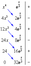
Now, multiply along the diagonals shown in the table. In front of each product put the sign in the third column that corresponds to the “\(u\)” term for that product. In this case this would give,
\[\begin{align*}\int{{{x^4}{{\bf{e}}^{\frac{x}{2}}}\,dx}} & = \left( {{x^4}} \right)\left( {2{{\bf{e}}^{\frac{x}{2}}}} \right) - \left( {4{x^3}} \right)\left( {4{{\bf{e}}^{\frac{x}{2}}}} \right) + \left( {12{x^2}} \right)\left( {8{{\bf{e}}^{\frac{x}{2}}}} \right) - \left( {24x} \right)\left( {16{{\bf{e}}^{\frac{x}{2}}}} \right) + \left( {24} \right)\left( {32{{\bf{e}}^{\frac{x}{2}}}} \right)\\ & = 2{x^4}{{\bf{e}}^{\frac{x}{2}}} - 16{x^3}{{\bf{e}}^{\frac{x}{2}}} + 96{x^2}{{\bf{e}}^{\frac{x}{2}}} - 384x{{\bf{e}}^{\frac{x}{2}}} + 768{{\bf{e}}^{\frac{x}{2}}} + c\end{align*}\]We’ve got the integral. This is much easier than writing down all the various \(u\)’s and \(dv\)’s that we’d have to do otherwise.
So, in this section we’ve seen how to do integration by parts. In your later math classes this is liable to be one of the more frequent integration techniques that you’ll encounter.
It is important to not get too locked into patterns that you may think you’ve seen. In most cases any pattern that you think you’ve seen can (and will be) violated at some point in time. Be careful!