Calculus I - Area and Volume Formulas

Show Mobile Notice Show All Notes Hide All Notes

Mobile Notice

You appear to be on a device with a "narrow" screen width (i.e. you are probably on a mobile phone). Due to the nature of the mathematics on this site it is best views in landscape mode. If your device is not in landscape mode many of the equations will run off the side of your device (should be able to scroll to see them) and some of the menu items will be cut off due to the narrow screen width.

Appendix A.6 : Area and Volume Formulas

In this section we will derive the formulas used to get the area between two curves and the volume of a solid of revolution.

Area Between Two Curves

We will start with the formula for determining the area between $y = f\left( x \right)$ and $y = g\left( x \right)$ on the interval $\left[ {a,b} \right]$. We will also assume that $f\left( x \right) \ge g\left( x \right)$ on $\left[ {a,b} \right]$.

We will now proceed much as we did when we looked that the Area Problem in the Integrals Chapter. We will first divide up the interval into $n$ equal subintervals each with length,

\[\Delta x = \frac{{b - a}}{n}\]

Next, pick a point in each subinterval, $x_i^*$, and we can then use rectangles on each interval as follows.

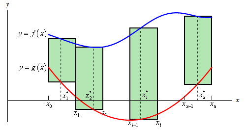
$This is the graph of two functions, f(x) and g(x), on the domain a<x<b. The graph of f(x) is always larger than the graph of g(x). Along the x-axis are points labeled $x_{0}$, $x_{1}$, $x_{2}$ on the left end $x_{i-1}$,$x_{i}$ in the middle and $x_{n-1}$, $x_{n}$ on the right end. Between each pair of points is another set of points labeled $x_{1}^{*}$, $x_{2}^{*}$, $x_{3}^{*}$ on the left $x_{i}^{*}$ in the middle and $x_{n}^{*}$ on the right. Each of the “*” points are used to get the height of a rectangle above it. So, there are two rectangles on the left one in the middle and one on the right that are used to represent the area between the two curves. The bottom of each rectangle is on g(x) and the top is on f(x).$

The height of each of these rectangles is given by,

\[f\left( {x_i^*} \right) - g\left( {x_i^*} \right)\]

and the area of each rectangle is then,

\[\left( {f\left( {x_i^*} \right) - g\left( {x_i^*} \right)} \right)\Delta x\]

So, the area between the two curves is then approximated by,

\[A \approx \sum\limits_{i = 1}^n {\left( {f\left( {x_i^*} \right) - g\left( {x_i^*} \right)} \right)\Delta x} \]

The exact area is,

\[A = \mathop {\lim }\limits_{n \to \infty } \sum\limits_{i = 1}^n {\left( {f\left( {x_i^*} \right) - g\left( {x_i^*} \right)} \right)\Delta x} \]

Now, recalling the definition of the definite integral this is nothing more than,

\[A = \int_{{\,a}}^{{\,b}}{{f\left( x \right) - g\left( x \right)\,dx}}\]

The formula above will work provided the two functions are in the form $y = f\left( x \right)$ and $y = g\left( x \right)$. However, not all functions are in that form.

Sometimes we will be forced to work with functions in the form between $x = f\left( y \right)$ and $x = g\left( y \right)$ on the interval $\left[ {c,d} \right]$ (an interval of $y$ values…). When this happens, the derivation is identical. First we will start by assuming that $f\left( y \right) \ge g\left( y \right)$ on $\left[ {c,d} \right]$. We can then divide up the interval into equal subintervals and build rectangles on each of these intervals. Here is a sketch of this situation.

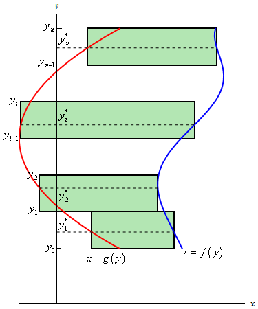
$This is the graph of two functions, f(y) and g(y), on the domain c<y<d. The graph of f(y) is always larger than the graph of g(y). Along the y-axis are points labeled $y_{0}$, $y_{1}$, $y_{2}$ on the left end $y_{i-1}$,$y_{i}$ in the middle and $y_{n-1}$, $y_{n}$ on the right end. Between each pair of points is another set of points labeled $y_{1}^{*}$, $y_{2}^{*}$, $y_{3}^{*}$ on the left $y_{i}^{*}$ in the middle and $xy_{n}^{*}$ on the right. Each of the “*” points are used to get the width of a rectangle along it. So, there are two rectangles on the bottom, one in the middle and one on the top that are used to represent the area between the two curves. The left side of each rectangle is on g(x) and the right side is on f(x).$

Following the work from above, we will arrive at the following for the area,

\[A = \int_{{\,c}}^{{\,d}}{{f\left( y \right) - g\left( y \right)\,dy}}\]

So, regardless of the form that the functions are in we use basically the same formula.

Volumes for Solid of Revolution

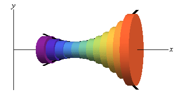
Before deriving the formula for this we should probably first define just what a solid of revolution is. To get a solid of revolution we start out with a function, $y = f\left( x \right)$, on an interval $\left[ {a,b} \right]$.

This is the graph of some unknown function on the domain a<x<b. It is completely in the 1st quadrant and looks like a parabola that opens upwards. The left end of the graph is lower than right end of the graph.

We then rotate this curve about a given axis to get the surface of the solid of revolution. For purposes of this derivation let’s rotate the curve about the $x$-axis. Doing this gives the following three dimensional region.

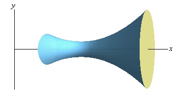
This is the graph of the solid we get from rotating the graph from above about the x-axis. It looks like an odd vase laying on its side. It has a wide “mouth” on the right side with a narrower “mouth” on the left side and an even narrow middle that corresponds to the vertex of the parabola from the graph.

We want to determine the volume of the interior of this object. To do this we will proceed much as we did for the area between two curves case. We will first divide up the interval into $n$ subintervals of width,

\[\Delta x = \frac{{b - a}}{n}\]

We will then choose a point from each subinterval, $x_i^*$.

Now, in the area between two curves case we approximated the area using rectangles on each subinterval. For volumes we will use disks on each subinterval to approximate the area. The area of the face of each disk is given by $A\left( {x_i^*} \right)$ and the volume of each disk is

\[{V_i} = A\left( {x_i^*} \right)\Delta x\]

Here is a sketch of this,

This is a sketch of the solid approximated by a series of 12 disks centered on the x-axis and whose edges are on the graph of the function defining the boundary of the solid.

The volume of the region can then be approximated by,

\[V \approx \sum\limits_{i = 1}^n {A\left( {x_i^*} \right)\Delta x} \]

The exact volume is then,

\[\begin{align*}V & = \mathop {\lim }\limits_{n \to \infty } \sum\limits_{i = 1}^n {A\left( {x_i^*} \right)\Delta x} \\ & = \int_{{\,a}}^{{\,b}}{{A\left( x \right)\,dx}}\end{align*}\]

So, in this case the volume will be the integral of the cross-sectional area at any $x$, $A\left( x \right)$. Note as well that, in this case, the cross-sectional area is a circle and we could go farther and get a formula for that as well. However, the formula above is more general and will work for any way of getting a cross section so we will leave it like it is.

In the sections where we actually use this formula we will also see that there are ways of generating the cross section that will actually give a cross-sectional area that is a function of $y$ instead of $x$. In these cases the formula will be,

\[V = \int_{{\,c}}^{{\,d}}{{A\left( y \right)\,dy}},\,\,\,\hspace{0.25in}c \le y \le d\]

In this case we looked at rotating a curve about the $x$-axis, however, we could have just as easily rotated the curve about the $y$-axis. In fact, we could rotate the curve about any vertical or horizontal axis and in all of these, case we can use one or both of the following formulas.

\[V = \int_{{\,a}}^{{\,b}}{{A\left( x \right)\,dx}}\hspace{0.25in}\hspace{0.25in}\hspace{0.25in}V = \int_{{\,c}}^{{\,d}}{{A\left( y \right)\,dy}}\]