Section 9.5 : Solving the Heat Equation
Okay, it is finally time to completely solve a partial differential equation. In the previous section we applied separation of variables to several partial differential equations and reduced the problem down to needing to solve two ordinary differential equations. In this section we will now solve those ordinary differential equations and use the results to get a solution to the partial differential equation. We will be concentrating on the heat equation in this section and will do the wave equation and Laplace’s equation in later sections.
The first problem that we’re going to look at will be the temperature distribution in a bar with zero temperature boundaries. We are going to do the work in a couple of steps so we can take our time and see how everything works.
The first thing that we need to do is find a solution that will satisfy the partial differential equation and the boundary conditions. At this point we will not worry about the initial condition. The solution we’ll get first will not satisfy the vast majority of initial conditions but as we’ll see it can be used to find a solution that will satisfy a sufficiently nice initial condition.
Okay the first thing we technically need to do here is apply separation of variables. Even though we did that in the previous section let’s recap here what we did.
First, we assume that the solution will take the form,
\[u\left( {x,t} \right) = \varphi \left( x \right)G\left( t \right)\]and we plug this into the partial differential equation and boundary conditions. We separate the equation to get a function of only \(t\) on one side and a function of only \(x\) on the other side and then introduce a separation constant. This leaves us with two ordinary differential equations.
We did all of this in Example 1 of the previous section and the two ordinary differential equations are,
\[\begin{align*}\frac{{dG}}{{dt}} = - k\lambda G\hspace{0.25in} & \frac{{{d^2}\varphi }}{{d{x^2}}} + \lambda \varphi = 0\\ & \varphi \left( 0 \right) = 0\hspace{0.25in}\varphi \left( L \right) = 0\end{align*}\]The time dependent equation can really be solved at any time, but since we don’t know what \(\lambda \) is yet let’s hold off on that one. Also note that in many problems only the boundary value problem can be solved at this point so don’t always expect to be able to solve either one at this point.
The spatial equation is a boundary value problem and we know from our work in the previous chapter that it will only have non-trivial solutions (which we want) for certain values of \(\lambda \), which we’ll recall are called eigenvalues. Once we have those we can determine the non-trivial solutions for each \(\lambda \), i.e. eigenfunctions.
Now, we actually solved the spatial problem,
\[\begin{align*}& \frac{{{d^2}\varphi }}{{d{x^2}}} + \lambda \varphi = 0\\ & \varphi \left( 0 \right) = 0\hspace{0.25in}\varphi \left( L \right) = 0\end{align*}\]in Example 1 of the Eigenvalues and Eigenfunctions section of the previous chapter for \(L = 2\pi \). So, because we’ve solved this once for a specific \(L\) and the work is not all that much different for a general \(L\) we’re not going to be putting in a lot of explanation here and if you need a reminder on how something works or why we did something go back to Example 1 from the Eigenvalues and Eigenfunctions section for a reminder.
We’ve got three cases to deal with so let’s get going.
\(\underline {\lambda > 0} \)
In this case we know the solution to the differential equation is,
Applying the first boundary condition gives,
\[0 = \varphi \left( 0 \right) = {c_1}\]Now applying the second boundary condition, and using the above result of course, gives,
\[0 = \varphi \left( L \right) = {c_2}\sin \left( {L\sqrt \lambda } \right)\]Now, we are after non-trivial solutions and so this means we must have,
\[\sin \left( {L\sqrt \lambda } \right) = 0\hspace{0.25in} \Rightarrow \hspace{0.25in}L\sqrt \lambda = n\pi \hspace{0.25in}n = 1,2,3, \ldots \]The positive eigenvalues and their corresponding eigenfunctions of this boundary value problem are then,
\[{\lambda _{\,n}} = {\left( {\frac{{n\pi }}{L}} \right)^2}\hspace{0.25in}{\varphi _n}\left( x \right) = \sin \left( {\frac{{n\,\pi \,x}}{L}} \right)\hspace{0.25in}n = 1,2,3, \ldots \]Note that we don’t need the \({c_2}\) in the eigenfunction as it will just get absorbed into another constant that we’ll be picking up later on.
\(\underline {\lambda = 0} \)
The solution to the differential equation in this case is,
Applying the boundary conditions gives,
\[0 = \varphi \left( 0 \right) = {c_1}\hspace{0.25in}0 = \varphi \left( L \right) = {c_2}L\hspace{0.25in} \Rightarrow \hspace{0.25in}{c_2} = 0\]So, in this case the only solution is the trivial solution and so \(\lambda = 0\) is not an eigenvalue for this boundary value problem.
\(\underline {\lambda < 0} \)
Here the solution to the differential equation is,
Applying the first boundary condition gives,
\[0 = \varphi \left( 0 \right) = {c_1}\]and applying the second gives,
\[0 = \varphi \left( L \right) = {c_2}\sinh \left( {L\sqrt { - \lambda } } \right)\]So, we are assuming \(\lambda < 0\) and so \(L\sqrt { - \lambda } \ne 0\) and this means \(\sinh \left( {L\sqrt { - \lambda } } \right) \ne 0\). We therefore we must have \({c_2} = 0\) and so we can only get the trivial solution in this case.
Therefore, there will be no negative eigenvalues for this boundary value problem.
The complete list of eigenvalues and eigenfunctions for this problem are then,
\[{\lambda _{\,n}} = {\left( {\frac{{n\pi }}{L}} \right)^2}\hspace{0.25in}{\varphi _n}\left( x \right) = \sin \left( {\frac{{n\,\pi \,x}}{L}} \right)\hspace{0.25in}n = 1,2,3, \ldots \]Now let’s solve the time differential equation,
\[\frac{{dG}}{{dt}} = - k{\lambda _n}G\]and note that even though we now know \(\lambda \) we’re not going to plug it in quite yet to keep the mess to a minimum. We will however now use \({\lambda _n}\) to remind us that we actually have an infinite number of possible values here.
This is a simple linear (and separable for that matter) 1st order differential equation and so we’ll let you verify that the solution is,
\[G\left( t \right) = c{{\bf{e}}^{ - k{\lambda _{\,n}}t}} = c{{\bf{e}}^{ - k{{\left( {\frac{{n\pi }}{L}} \right)}^2}\,t}}\]Okay, now that we’ve gotten both of the ordinary differential equations solved we can finally write down a solution. Note however that we have in fact found infinitely many solutions since there are infinitely many solutions (i.e. eigenfunctions) to the spatial problem.
Our product solution are then,
\[{u_n}\left( {x,t} \right) = {B_n}\sin \left( {\frac{{n\pi x}}{L}} \right){{\bf{e}}^{ - k{{\left( {\frac{{n\pi }}{L}} \right)}^2}\,t}}\hspace{0.25in}n = 1,2,3, \ldots \]We’ve denoted the product solution \({u_n}\) to acknowledge that each value of \(n\) will yield a different solution. Also note that we’ve changed the \(c\) in the solution to the time problem to \({B_n}\) to denote the fact that it will probably be different for each value of \(n\) as well and because had we kept the \({c_2}\) with the eigenfunction we’d have absorbed it into the \(c\) to get a single constant in our solution.
So, there we have it. The function above will satisfy the heat equation and the boundary condition of zero temperature on the ends of the bar.
The problem with this solution is that it simply will not satisfy almost every possible initial condition we could possibly want to use. That does not mean however, that there aren’t at least a few that it will satisfy as the next example illustrates.
- \(\displaystyle f\left( x \right) = 6\sin \left( {\frac{{\pi x}}{L}} \right)\)
- \(\displaystyle f\left( x \right) = 12\sin \left( {\frac{{9\pi x}}{L}} \right) - 7\sin \left( {\frac{{4\pi x}}{L}} \right)\)
This is actually easier than it looks like. All we need to do is choose \(n = 1\) and \({B_1} = 6\) in the product solution above to get,
\[u\left( {x,t} \right) = 6\sin \left( {\frac{{\pi x}}{L}} \right){{\bf{e}}^{ - k{{\left( {\frac{\pi }{L}} \right)}^2}\,t}}\]and we’ve got the solution we need. This is a product solution for the first example and so satisfies the partial differential equation and boundary conditions and will satisfy the initial condition since plugging in \(t = 0\) will drop out the exponential.
b \(\displaystyle f\left( x \right) = 12\sin \left( {\frac{{9\pi x}}{L}} \right) - 7\sin \left( {\frac{{4\pi x}}{L}} \right)\) Show Solution
This is almost as simple as the first part. Recall from the Principle of Superposition that if we have two solutions to a linear homogeneous differential equation (which we’ve got here) then their sum is also a solution. So, all we need to do is choose \(n\) and \({B_n}\) as we did in the first part to get a solution that satisfies each part of the initial condition and then add them up. Doing this gives,
\[u\left( {x,t} \right) = 12\sin \left( {\frac{{9\pi x}}{L}} \right){{\bf{e}}^{ - k{{\left( {\frac{{9\pi }}{L}} \right)}^2}\,t}} - 7\sin \left( {\frac{{4\pi x}}{L}} \right){{\bf{e}}^{ - k{{\left( {\frac{{4\pi }}{L}} \right)}^2}\,t}}\]We’ll leave it to you to verify that this does in fact satisfy the initial condition and the boundary conditions.
So, we’ve seen that our solution from the first example will satisfy at least a small number of highly specific initial conditions.
Now, let’s extend the idea out that we used in the second part of the previous example a little to see how we can get a solution that will satisfy any sufficiently nice initial condition. The Principle of Superposition is, of course, not restricted to only two solutions. For instance, the following is also a solution to the partial differential equation.
\[u\left( {x,t} \right) = \sum\limits_{n = 1}^M {{B_n}\sin \left( {\frac{{n\pi x}}{L}} \right){{\bf{e}}^{ - k{{\left( {\frac{{n\pi }}{L}} \right)}^2}\,t}}} \]and notice that this solution will not only satisfy the boundary conditions but it will also satisfy the initial condition,
\[u\left( {x,0} \right) = \sum\limits_{n = 1}^M {{B_n}\sin \left( {\frac{{n\pi x}}{L}} \right)} \]Let’s extend this out even further and take the limit as \(M \to \infty \). Doing this our solution now becomes,
\[u\left( {x,t} \right) = \sum\limits_{n = 1}^\infty {{B_n}\sin \left( {\frac{{n\pi x}}{L}} \right){{\bf{e}}^{ - k{{\left( {\frac{{n\pi }}{L}} \right)}^2}\,t}}} \]This solution will satisfy any initial condition that can be written in the form,
\[u\left( {x,0} \right) = f\left( x \right) = \sum\limits_{n = 1}^\infty {{B_n}\sin \left( {\frac{{n\pi x}}{L}} \right)} \]This may still seem to be very restrictive, but the series on the right should look awful familiar to you after the previous chapter. The series on the left is exactly the Fourier sine series we looked at in that chapter. Also recall that when we can write down the Fourier sine series for any piecewise smooth function on \(0 \le x \le L\).
So, provided our initial condition is piecewise smooth after applying the initial condition to our solution we can determine the \({B_n}\) as if we were finding the Fourier sine series of initial condition. So we can either proceed as we did in that section and use the orthogonality of the sines to derive them or we can acknowledge that we’ve already done that work and know that coefficients are given by,
\[{B_n} = \frac{2}{L}\int_{{\,0}}^{{\,L}}{{f\left( x \right)\sin \left( {\frac{{n\,\pi x}}{L}} \right)\,dx}}\,\,\,\,\,\,\,n = 1,2,3, \ldots \]So, we finally can completely solve a partial differential equation.
There isn’t really all that much to do here as we’ve done most of it in the examples and discussion above.
First, the solution is,
\[u\left( {x,t} \right) = \sum\limits_{n = 1}^\infty {{B_n}\sin \left( {\frac{{n\pi x}}{L}} \right){{\bf{e}}^{ - k{{\left( {\frac{{n\pi }}{L}} \right)}^2}\,t}}} \]The coefficients are given by,
\[{B_n} = \frac{2}{L}\int_{{\,0}}^{{\,L}}{{20\sin \left( {\frac{{n\,\pi x}}{L}} \right)\,dx}} = \frac{2}{L}\left( {\frac{{20L\left( {1 - \cos \left( {n\pi } \right)} \right)}}{{n\pi }}} \right) = \frac{{40\left( {1 - {{\left( { - 1} \right)}^n}} \right)}}{{n\pi }}\]If we plug these in we get the solution,
\[u\left( {x,t} \right) = \sum\limits_{n = 1}^\infty {\frac{{40\left( {1 - \,{{\left( { - 1} \right)}^n}} \right)}}{{n\,\pi }}\sin \left( {\frac{{n\pi x}}{L}} \right){{\bf{e}}^{ - k{{\left( {\frac{{n\pi }}{L}} \right)}^2}\,t}}} \]That almost seems anti-climactic. This was a very short problem. Of course, some of that came about because we had a really simple constant initial condition and so the integral was very simple. However, don’t forget all the work that we had to put into discussing Fourier sine series, solving boundary value problems, applying separation of variables and then putting all of that together to reach this point.
While the example itself was very simple, it was only simple because of all the work that we had to put into developing the ideas that even allowed us to do this. Because of how “simple” it will often be to actually get these solutions we’re not actually going to do anymore with specific initial conditions. We will instead concentrate on simply developing the formulas that we’d be required to evaluate in order to get an actual solution.
So, having said that let’s move onto the next example. In this case we’re going to again look at the temperature distribution in a bar with perfectly insulated boundaries. We are also no longer going to go in steps. We will do the full solution as a single example and end up with a solution that will satisfy any piecewise smooth initial condition.
We applied separation of variables to this problem in Example 2 of the previous section. So, after assuming that our solution is in the form,
\[u\left( {x,t} \right) = \varphi \left( x \right)G\left( t \right)\]and applying separation of variables we get the following two ordinary differential equations that we need to solve.
\[\begin{align*}\frac{{dG}}{{dt}} = - k\lambda G\hspace{0.25in} & \frac{{{d^2}\varphi }}{{d{x^2}}} + \lambda \varphi = 0\\ & \frac{{d\varphi }}{{dx}}\left( 0 \right) = 0\hspace{0.25in}\frac{{d\varphi }}{{dx}}\left( L \right) = 0\end{align*}\]We solved the boundary value problem in Example 2 of the Eigenvalues and Eigenfunctions section of the previous chapter for \(L = 2\pi \) so as with the first example in this section we’re not going to put a lot of explanation into the work here. If you need a reminder on how this works go back to the previous chapter and review the example we worked there. Let’s get going on the three cases we’ve got to work for this problem.
\(\underline {\lambda > 0} \)
The solution to the differential equation is,
Applying the first boundary condition gives,
\[0 = \frac{{d\varphi }}{{dx}}\left( 0 \right) = \sqrt \lambda \,{c_2}\hspace{0.25in} \Rightarrow \hspace{0.25in}{c_2} = 0\]The second boundary condition gives,
\[0 = \frac{{d\varphi }}{{dx}}\left( L \right) = - \sqrt \lambda \,{c_1}\sin \left( {L\sqrt \lambda } \right)\]Recall that \(\lambda > 0\) and so we will only get non-trivial solutions if we require that,
\[\sin \left( {L\sqrt \lambda } \right) = 0\hspace{0.25in} \Rightarrow \hspace{0.25in}L\sqrt \lambda = n\pi \hspace{0.25in}n = 1,2,3, \ldots \]The positive eigenvalues and their corresponding eigenfunctions of this boundary value problem are then,
\[{\lambda _{\,n}} = {\left( {\frac{{n\pi }}{L}} \right)^2}\hspace{0.25in}{\varphi _n}\left( x \right) = \cos \left( {\frac{{n\,\pi x}}{L}} \right)\hspace{0.25in}n = 1,2,3, \ldots \]\(\underline {\lambda = 0} \)
The general solution is,
Applying the first boundary condition gives,
\[0 = \frac{{d\varphi }}{{dx}}\left( 0 \right) = {c_2}\]Using this the general solution is then,
\[\varphi \left( x \right) = {c_1}\]and note that this will trivially satisfy the second boundary condition. Therefore \(\lambda = 0\) is an eigenvalue for this BVP and the eigenfunctions corresponding to this eigenvalue is,
\[\varphi \left( x \right) = 1\]\(\underline {\lambda < 0} \)
The general solution here is,
Applying the first boundary condition gives,
\[0 = \frac{{d\varphi }}{{dx}}\left( 0 \right) = \sqrt { - \lambda } \,{c_2}\hspace{0.25in} \Rightarrow \hspace{0.25in}{c_2} = 0\]The second boundary condition gives,
\[0 = \frac{{d\varphi }}{{dx}}\left( L \right) = \sqrt { - \lambda } \,{c_1}\sinh \left( {L\sqrt { - \lambda } } \right)\]We know that \(L\sqrt { - \lambda } \ne 0\) and so \(\sinh \left( {L\sqrt { - \lambda } } \right) \ne 0\). Therefore, we must have \({c_1} = 0\) and so, this boundary value problem will have no negative eigenvalues.
So, the complete list of eigenvalues and eigenfunctions for this problem is then,
\[\begin{align*}{\lambda _{\,n}} & = {\left( {\frac{{n\pi }}{L}} \right)^2} & \hspace{0.25in}{\varphi _n}\left( x \right) & = \cos \left( {\frac{{n\,\pi x}}{L}} \right)\hspace{0.25in}n = 1,2,3, \ldots \\ {\lambda _{\,0}} & = 0 & \hspace{0.25in}{\varphi _0}\left( x \right) & = 1\end{align*}\]and notice that we get the \({\lambda _{\,0}} = 0\) eigenvalue and its eigenfunction if we allow \(n = 0\) in the first set and so we’ll use the following as our set of eigenvalues and eigenfunctions.
\[{\lambda _{\,n}} = {\left( {\frac{{n\pi }}{L}} \right)^2}\hspace{0.25in}{\varphi _n}\left( x \right) = \cos \left( {\frac{{n\,\pi x}}{L}} \right)\hspace{0.25in}n = 0,1,2,3, \ldots \]The time problem here is identical to the first problem we looked at so,
\[G\left( t \right) = c{{\bf{e}}^{ - k{{\left( {\frac{{n\pi }}{L}} \right)}^2}\,t}}\]Our product solutions will then be,
\[{u_n}\left( {x,t} \right) = {A_n}\cos \left( {\frac{{n\pi x}}{L}} \right){{\bf{e}}^{ - k{{\left( {\frac{{n\pi }}{L}} \right)}^2}\,t}}\hspace{0.25in}n = 0,1,2,3, \ldots \]and the solution to this partial differential equation is,
\[u\left( {x,t} \right) = \sum\limits_{n = 0}^\infty {{A_n}\cos \left( {\frac{{n\pi x}}{L}} \right){{\bf{e}}^{ - k{{\left( {\frac{{n\pi }}{L}} \right)}^2}\,t}}} \]If we apply the initial condition to this we get,
\[u\left( {x,0} \right) = f\left( x \right) = \sum\limits_{n = 0}^\infty {{A_n}\cos \left( {\frac{{n\,\pi x}}{L}} \right)} \]and we can see that this is nothing more than the Fourier cosine series for \(f\left( x \right)\)on \(0 \le x \le L\) and so again we could use the orthogonality of the cosines to derive the coefficients or we could recall that we’ve already done that in the previous chapter and know that the coefficients are given by,
\[{A_n} = \left\{ {\begin{array}{*{20}{l}}{\frac{1}{L}\int_{{\,0}}^{{\,L}}{{f\left( x \right)\,dx}}}&{\,\,\,\,\,n = 0}\\{\frac{2}{L}\int_{{\,0}}^{{\,L}}{{f\left( x \right)\cos \left( {\frac{{n\,\pi x}}{L}} \right)\,dx}}}&{\,\,\,\,\,n \ne 0}\end{array}} \right.\]The last example that we’re going to work in this section is a little different from the first two. We are going to consider the temperature distribution in a thin circular ring. We will consider the lateral surfaces to be perfectly insulated and we are also going to assume that the ring is thin enough so that the temperature does not vary with distance from the center of the ring.
So, what does that leave us with? Let’s set \(x = 0\) as shown below and then let \(x\) be the arc length of the ring as measured from this point.
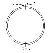
We will measure \(x\) as positive if we move to the right and negative if we move to the left of \(x = 0\). This means that at the top of the ring we’ll meet where \(x = L\) (if we move to the right) and \(x = - L\) (if we move to the left). By doing this we can consider this ring to be a bar of length 2\(L\) and the heat equation that we developed earlier in this chapter will still hold.
At the point of the ring we consider the two “ends” to be in perfect thermal contact. This means that at the two ends both the temperature and the heat flux must be equal. In other words we must have,
\[u\left( { - L,t} \right) = u\left( {L,t} \right)\hspace{0.25in}\frac{{\partial u}}{{\partial x}}\left( { - L,t} \right) = \frac{{\partial u}}{{\partial x}}\left( {L,t} \right)\]If you recall from the section in which we derived the heat equation we called these periodic boundary conditions. So, the problem we need to solve to get the temperature distribution in this case is,
We applied separation of variables to this problem in Example 3 of the previous section. So, if we assume the solution is in the form,
\[u\left( {x,t} \right) = \varphi \left( x \right)G\left( t \right)\]we get the following two ordinary differential equations that we need to solve.
\[\begin{align*}\frac{{dG}}{{dt}} = - k\lambda G\hspace{0.25in} & \frac{{{d^2}\varphi }}{{d{x^2}}} + \lambda \varphi = 0\\ & \varphi \left( { - L} \right) = \varphi \left( L \right)\hspace{0.25in}\frac{{d\varphi }}{{dx}}\left( { - L} \right) = \frac{{d\varphi }}{{dx}}\left( L \right)\end{align*}\]As we’ve seen with the previous two problems we’ve already solved a boundary value problem like this one back in the Eigenvalues and Eigenfunctions section of the previous chapter, Example 3 to be exact with \(L = \pi \). So, if you need a little more explanation of what’s going on here go back to this example and you can see a little more explanation.
We again have three cases to deal with here.
\(\underline {\lambda > 0} \)
The general solution to the differential equation is,
Applying the first boundary condition and recalling that cosine is an even function and sine is an odd function gives us,
\[\begin{align*}{c_1}\cos \left( { - L\sqrt \lambda } \right) + {c_2}\sin \left( { - L\sqrt \lambda } \right)& = {c_1}\cos \left( {L\sqrt \lambda } \right) + {c_2}\sin \left( {L\sqrt \lambda } \right)\\ - {c_2}\sin \left( {L\sqrt \lambda } \right) & = {c_2}\sin \left( {L\sqrt \lambda } \right)\\ 0 & = 2{c_2}\sin \left( {L\sqrt \lambda } \right)\end{align*}\]At this stage we can’t really say anything as either \({c_2}\) or sine could be zero. So, let’s apply the second boundary condition and see what we get.
\[\begin{align*} - \sqrt \lambda \,{c_1}\sin \left( { - L\sqrt \lambda } \right) + \sqrt \lambda \,{c_2}\cos \left( { - L\sqrt \lambda } \right) & = - \sqrt \lambda \,{c_1}\sin \left( {L\sqrt \lambda } \right) + \sqrt \lambda \,{c_2}\cos \left( {L\sqrt \lambda } \right)\\ \sqrt \lambda \,{c_1}\sin \left( {L\sqrt \lambda } \right) & = - \sqrt \lambda \,{c_1}\sin \left( {L\sqrt \lambda } \right)\\ 2\sqrt \lambda \,{c_1}\sin \left( {L\sqrt \lambda } \right) & = 0\end{align*}\]We get something similar. However, notice that if \(\sin \left( {L\sqrt \lambda } \right) \ne 0\) then we would be forced to have \({c_1} = {c_2} = 0\) and this would give us the trivial solution which we don’t want.
This means therefore that we must have \(\sin \left( {L\sqrt \lambda } \right) = 0\) which in turn means (from work in our previous examples) that the positive eigenvalues for this problem are,
\[{\lambda _{\,n}} = {\left( {\frac{{n\pi }}{L}} \right)^2}\hspace{0.25in}n = 1,2,3, \ldots \]Now, there is no reason to believe that \({c_1} = 0\) or \({c_2} = 0\). All we know is that they both can’t be zero and so that means that we in fact have two sets of eigenfunctions for this problem corresponding to positive eigenvalues. They are,
\[{\varphi _n}\left( x \right) = \cos \left( {\frac{{n\pi x}}{L}} \right)\hspace{0.25in}{\varphi _n}\left( x \right) = \sin \left( {\frac{{n\pi x}}{L}} \right)\hspace{0.25in}n = 1,2,3, \ldots \]\(\underline {\lambda = 0} \)
The general solution in this case is,
Applying the first boundary condition gives,
\[\begin{align*}{c_1} + {c_2}\left( { - L} \right) & = {c_1} + {c_2}\left( L \right)\\ 2L{c_2} & = 0\hspace{0.25in} \Rightarrow \hspace{0.25in}{c_2} = 0\end{align*}\]The general solution is then,
\[\varphi \left( x \right) = {c_1}\]and this will trivially satisfy the second boundary condition. Therefore \(\lambda = 0\) is an eigenvalue for this BVP and the eigenfunctions corresponding to this eigenvalue is,
\[\varphi \left( x \right) = 1\]\(\underline {\lambda < 0} \)
For this final case the general solution here is,
Applying the first boundary condition and using the fact that hyperbolic cosine is even and hyperbolic sine is odd gives,
\[\begin{align*}{c_1}\cosh \left( { - L\sqrt { - \lambda } } \right) + {c_2}\sinh \left( { - L\sqrt { - \lambda } } \right) & = {c_1}\cosh \left( {L\sqrt { - \lambda } } \right) + {c_2}\sinh \left( {L\sqrt { - \lambda } } \right)\\ - {c_2}\sinh \left( { - L\sqrt { - \lambda } } \right) & = {c_2}\sinh \left( {L\sqrt { - \lambda } } \right)\\ 2{c_2}\sinh \left( {L\sqrt { - \lambda } } \right) & = 0\end{align*}\]Now, in this case we are assuming that \(\lambda < 0\) and so \(L\sqrt { - \lambda } \ne 0\). This turn tells us that \(\sinh \left( {L\sqrt { - \lambda } } \right) \ne 0\). We therefore must have \({c_2} = 0\).
Let’s now apply the second boundary condition to get,
\[\begin{align*}\sqrt { - \lambda } \,{c_1}\sinh \left( { - L\sqrt { - \lambda } } \right) & = \sqrt { - \lambda } \,{c_1}\sinh \left( {L\sqrt { - \lambda } } \right)\\ 2\sqrt { - \lambda } \,{c_1}\sinh \left( {L\sqrt { - \lambda } } \right) & = 0\hspace{0.25in} \Rightarrow \hspace{0.25in}{c_1} = 0\end{align*}\]By our assumption on \(\lambda \) we again have no choice here but to have \({c_1} = 0\) and so for this boundary value problem there are no negative eigenvalues.
Summarizing up then we have the following sets of eigenvalues and eigenfunctions and note that we’ve merged the \(\lambda = 0\) case into the cosine case since it can be here to simplify things up a little.
\[\begin{align*}{\lambda _{\,n}} & = {\left( {\frac{{n\pi }}{L}} \right)^2} & \hspace{0.25in}{\varphi _n}\left( x \right) & = \cos \left( {\frac{{n\,\pi x}}{L}} \right)\hspace{0.25in}n = 0,1,2,3, \ldots \\ {\lambda _{\,n}} & = {\left( {\frac{{n\pi }}{L}} \right)^2} & \hspace{0.25in}{\varphi _n}\left( x \right) & = \sin \left( {\frac{{n\,\pi x}}{L}} \right)\hspace{0.25in}n = 1,2,3, \ldots \end{align*}\]The time problem is again identical to the two we’ve already worked here and so we have,
\[G\left( t \right) = c{{\bf{e}}^{ - k{{\left( {\frac{{n\pi }}{L}} \right)}^2}\,t}}\]Now, this example is a little different from the previous two heat problems that we’ve looked at. In this case we actually have two different possible product solutions that will satisfy the partial differential equation and the boundary conditions. They are,
\[\begin{align*}{u_n}\left( {x,t} \right) & = {A_n}\cos \left( {\frac{{n\pi x}}{L}} \right){{\bf{e}}^{ - k{{\left( {\frac{{n\pi }}{L}} \right)}^2}\,t}}\hspace{0.25in}n = 0,1,2,3, \ldots \\ {u_n}\left( {x,t} \right) & = {B_n}\sin \left( {\frac{{n\pi x}}{L}} \right){{\bf{e}}^{ - k{{\left( {\frac{{n\pi }}{L}} \right)}^2}\,t}}\hspace{0.25in}n = 1,2,3, \ldots \end{align*}\]The Principle of Superposition is still valid however and so a sum of any of these will also be a solution and so the solution to this partial differential equation is,
\[u\left( {x,t} \right) = \sum\limits_{n = 0}^\infty {{A_n}\cos \left( {\frac{{n\pi x}}{L}} \right){{\bf{e}}^{ - k{{\left( {\frac{{n\pi }}{L}} \right)}^2}\,t}}} + \sum\limits_{n = 1}^\infty {{B_n}\sin \left( {\frac{{n\pi x}}{L}} \right){{\bf{e}}^{ - k{{\left( {\frac{{n\pi }}{L}} \right)}^2}\,t}}} \]If we apply the initial condition to this we get,
\[u\left( {x,0} \right) = f\left( x \right) = \sum\limits_{n = 0}^\infty {{A_n}\cos \left( {\frac{{n\pi x}}{L}} \right)} + \sum\limits_{n = 1}^\infty {{B_n}\sin \left( {\frac{{n\pi x}}{L}} \right)} \]and just as we saw in the previous two examples we get a Fourier series. The difference this time is that we get the full Fourier series for a piecewise smooth initial condition on \( - L \le x \le L\). As noted for the previous two examples we could either rederive formulas for the coefficients using the orthogonality of the sines and cosines or we can recall the work we’ve already done. There’s really no reason at this point to redo work already done so the coefficients are given by,
\[\begin{align*}{A_0} & = \frac{1}{{2L}}\int_{{\, - L}}^{L}{{f\left( x \right)\,dx}}\\ {A_n} & = \frac{1}{L}\int_{{\, - L}}^{L}{{f\left( x \right)\cos \left( {\frac{{n\,\pi x}}{L}} \right)\,dx}}\hspace{0.25in}n = 1,2,3, \ldots \\ {B_n} & = \frac{1}{L}\int_{{\, - L}}^{L}{{f\left( x \right)\sin \left( {\frac{{n\,\pi x}}{L}} \right)\,dx}}\hspace{0.25in}n = 1,2,3, \ldots \end{align*}\]Note that this is the reason for setting up \(x\) as we did at the start of this problem. A full Fourier series needs an interval of \( - L \le x \le L\) whereas the Fourier sine and cosines series we saw in the first two problems need \(0 \le x \le L\).
Okay, we’ve now seen three heat equation problems solved and so we’ll leave this section. You might want to go through and do the two cases where we have a zero temperature on one boundary and a perfectly insulated boundary on the other to see if you’ve got this process down.