Calculus I - Area Problem

Show Mobile Notice Show All Notes Hide All Notes

Mobile Notice

You appear to be on a device with a "narrow" screen width (i.e. you are probably on a mobile phone). Due to the nature of the mathematics on this site it is best views in landscape mode. If your device is not in landscape mode many of the equations will run off the side of your device (should be able to scroll to see them) and some of the menu items will be cut off due to the narrow screen width.

Section 5.5 : Area Problem

As noted in the first section of this section there are two kinds of integrals and to this point we’ve looked at indefinite integrals. It is now time to start thinking about the second kind of integral : Definite Integrals. However, before we do that we’re going to take a look at the Area Problem. The area problem is to definite integrals what the tangent and rate of change problems are to derivatives.

The area problem will give us one of the interpretations of a definite integral and it will lead us to the definition of the definite integral.

To start off we are going to assume that we’ve got a function $f\left( x \right)$ that is positive on some interval $\left[ {a,b} \right]$. What we want to do is determine the area of the region between the function and the $x$-axis.

It’s probably easiest to see how we do this with an example. So, let’s determine the area between $f\left( x \right) = {x^2} + 1$ on $\left[ {0,2} \right]$. In other words, we want to determine the area of the shaded region below.

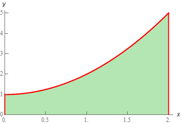
Now, at this point, we can’t do this exactly. However, we can estimate the area. We will estimate the area by dividing up the interval into $n$ subintervals each of width,

\[\Delta x = \frac{{b - a}}{n}\]

Then in each interval we can form a rectangle whose height is given by the function value at a specific point in the interval. We can then find the area of each of these rectangles, add them up and this will be an estimate of the area.

It’s probably easier to see this with a sketch of the situation. So, let’s divide up the interval into 4 subintervals and use the function value at the right endpoint of each interval to define the height of the rectangle. This gives,

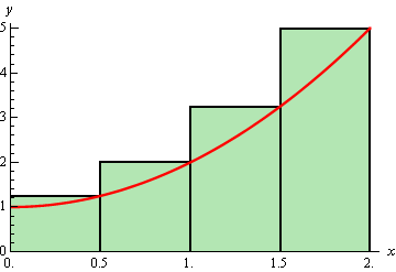
$The graph of $f\left( x \right)={{x}^{2}}+1$ on the domain 0<x<2. Also on the graph are four rectangles of width 1/2 whose bases are all on the x-axis and whose height goes up to the function graph on the right side of the rectangle.$

Note that by choosing the height as we did each of the rectangles will over estimate the area since each rectangle takes in more area than the graph each time. Now let’s estimate the area. First, the width of each of the rectangles is $\frac{1}{2}$. The height of each rectangle is determined by the function value at the right endpoint and so the height of each rectangle is nothing more that the function value at the right endpoint. Here is the estimated area.

\[\begin{align*}{A_{\,r}} & = \frac{1}{2}f\left( {\frac{1}{2}} \right) + \frac{1}{2}f\left( 1 \right) + \frac{1}{2}f\left( {\frac{3}{2}} \right) + \frac{1}{2}f\left( 2 \right)\\ & = \frac{1}{2}\left( {\frac{5}{4}} \right) + \frac{1}{2}\left( 2 \right) + \frac{1}{2}\left( {\frac{{13}}{4}} \right) + \frac{1}{2}\left( 5 \right)\\ & = 5.75\end{align*}\]

Of course, taking the rectangle heights to be the function value at the right endpoint is not our only option. We could have taken the rectangle heights to be the function value at the left endpoint. Using the left endpoints as the heights of the rectangles will give the following graph and estimated area.

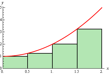
\[\begin{align*}{A_{\,l}} & = \frac{1}{2}f\left( 0 \right) + \frac{1}{2}f\left( {\frac{1}{2}} \right) + \frac{1}{2}f\left( 1 \right) + \frac{1}{2}f\left( {\frac{3}{2}} \right)\\ & = \frac{1}{2}\left( 1 \right) + \frac{1}{2}\left( {\frac{5}{4}} \right) + \frac{1}{2}\left( 2 \right) + \frac{1}{2}\left( {\frac{{13}}{4}} \right)\\ & = 3.75\end{align*}\]

In this case we can see that the estimation will be an underestimation since each rectangle misses some of the area each time.

There is one more common point for getting the heights of the rectangles that is often more accurate. Instead of using the right or left endpoints of each sub interval we could take the midpoint of each subinterval as the height of each rectangle. Here is the graph for this case.

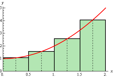
So, it looks like each rectangle will over and under estimate the area. This means that the approximation this time should be much better than the previous two choices of points. Here is the estimation for this case.

\[\begin{align*}{A_{\,m}} & = \frac{1}{2}f\left( {\frac{1}{4}} \right) + \frac{1}{2}f\left( {\frac{3}{4}} \right) + \frac{1}{2}f\left( {\frac{5}{4}} \right) + \frac{1}{2}f\left( {\frac{7}{4}} \right)\\ & = \frac{1}{2}\left( {\frac{{17}}{{16}}} \right) + \frac{1}{2}\left( {\frac{{25}}{{16}}} \right) + \frac{1}{2}\left( {\frac{{41}}{{16}}} \right) + \frac{1}{2}\left( {\frac{{65}}{{16}}} \right)\\ & = 4.625\end{align*}\]

We’ve now got three estimates. For comparison’s sake the exact area is

\[A = \frac{{14}}{3} = 4.66\overline{6}\]

So, both the right and left endpoint estimation did not do all that great of a job at the estimation. The midpoint estimation however did quite well.

Be careful to not draw any conclusion about how choosing each of the points will affect our estimation. In this case, because we are working with an increasing function choosing the right endpoints will overestimate and choosing left endpoint will underestimate.

If we were to work with a decreasing function we would get the opposite results. For decreasing functions the right endpoints will underestimate and the left endpoints will overestimate.

Also, if we had a function that both increased and decreased in the interval we would, in all likelihood, not even be able to determine if we would get an overestimation or underestimation.

Now, let’s suppose that we want a better estimation, because none of the estimations above really did all that great of a job at estimating the area. We could try to find a different point to use for the height of each rectangle but that would be cumbersome and there wouldn’t be any guarantee that the estimation would in fact be better. Also, we would like a method for getting better approximations that would work for any function we would chose to work with and if we just pick new points that may not work for other functions.

The easiest way to get a better approximation is to take more rectangles (i.e. increase $n$). Let’s double the number of rectangles that we used and see what happens. Here are the graphs showing the eight rectangles and the estimations for each of the three choices for rectangle heights that we used above.

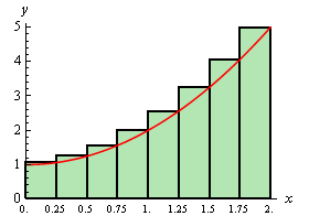
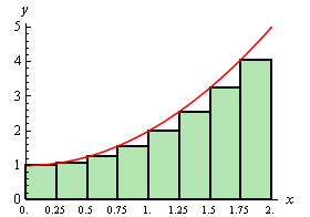
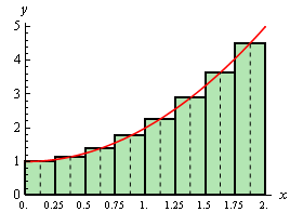
$The graph of $f\left( x \right)={{x}^{2}}+1$ on the domain 0<x<2. Also on the graph are eight rectangles of width 1/4 whose bases are all on the x-axis and whose height goes up to the function graph on the right side of the rectangle.$ $The graph of $f\left( x \right)={{x}^{2}}+1$ on the domain 0<x<2. Also on the graph are eight rectangles of width 1/4 whose bases are all on the x-axis and whose height goes up to the function graph on the left side of the rectangle.$

Here are the area estimations for each of these cases.

\[{A_{\,r}} = 5.1875\hspace{0.25in}\hspace{0.25in}{A_{\,l}} = 4.1875\hspace{0.25in}\hspace{0.25in}{A_{\,m}} = 4.65625\]

So, increasing the number of rectangles did improve the accuracy of the estimation as we’d guessed that it would.

Let’s work a slightly more complicated example.

Example 1 Estimate the area between $f\left( x \right) = {x^3} - 5{x^2} + 6x + 5$ and the $x$-axis on $\left[ {0,4} \right]$ using $n = 5$ subintervals and all three cases above for the heights of each rectangle.

Show Solution

First, let’s get the graph to make sure that the function is positive.

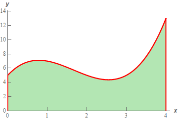
So, the graph is positive and the width of each subinterval will be,

\[\Delta x = \frac{4}{5} = 0.8\]

This means that the endpoints of the subintervals are,

\[0,\,\,\,0.8,\,\,\,1.6,\,\,\,2.4,\,\,\,3.2,\,\,\,4\,\]

Let’s first look at using the right endpoints for the function height. Here is the graph for this case.

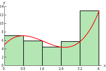
$The graph of $f\left( x \right)={{x}^{3}}-5{{x}^{2}}+6x+5$ on the domain 0<x<4 using 5 rectangles and right endpoints for the rectangle heights. Counting rectangles from left to right we get that rectangles 1, 4 and 5 all over estimate the area and rectangles 2 and 3 both underestimate the area.$

Notice, that unlike the first area we looked at, the choosing the right endpoints here will both over and underestimate the area depending on where we are on the curve. This will often be the case with a more general curve that the one we initially looked at. The area estimation using the right endpoints of each interval for the rectangle height is,

\[\begin{align*}{A_{\,r}} & = 0.8f\left( {0.8} \right) + 0.8f\left( {1.6} \right) + 0.8f\left( {2.4} \right) + 0.8f\left( {3.2} \right) + 0.8f\left( 4 \right)\\ & = 28.96\end{align*}\]

Now let’s take a look at left endpoints for the function height. Here is the graph.

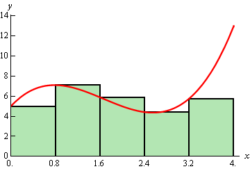
$The graph of $f\left( x \right)={{x}^{3}}-5{{x}^{2}}+6x+5$ on the domain 0<x<4 using 5 rectangles and left endpoints for the rectangle heights. Counting rectangles from left to right we get that rectangles 1, 4 and 5 all underestimate the area and rectangles 2 and 3 both overestimate the area.$

The area estimation using the left endpoints of each interval for the rectangle height is,

\[\begin{align*}{A_{\,l}} & = 0.8f\left( 0 \right) + 0.8f\left( {0.8} \right) + 0.8f\left( {1.6} \right) + 0.8f\left( {2.4} \right) + 0.8f\left( {3.2} \right)\\ & = 22.56\end{align*}\]

Finally, let’s take a look at the midpoints for the heights of each rectangle. Here is the graph,

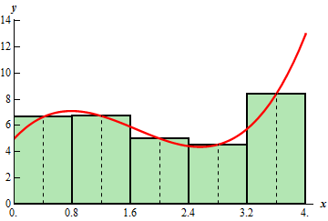
$The graph of $f\left( x \right)={{x}^{3}}-5{{x}^{2}}+6x+5$ on the domain 0<x<4 using 5 rectangles and midpoints for the rectangle heights. Each rectangle both over and underestimates the area.$

The area estimation using the midpoint is then,

\[\begin{align*}{A_{\,m}} & = 0.8f\left( {0.4} \right) + 0.8f\left( {1.2} \right) + 0.8f\left( 2 \right) + 0.8f\left( {2.8} \right) + 0.8f\left( {3.6} \right)\\ & = 25.12\end{align*}\]

For comparison purposes the exact area is,

\[A = \frac{{76}}{3} = 25.33\overline{3}\]

So, again the midpoint did a better job than the other two. While this will be the case more often than not, it won’t always be the case and so don’t expect this to always happen.

Now, let’s move on to the general case. Let’s start out with $f\left( x \right) \ge 0$ on $\left[ {a,b} \right]$ and we’ll divide the interval into $n$ subintervals each of length,

\[\Delta x = \frac{{b - a}}{n}\]

Note that the subintervals don’t have to be equal length, but it will make our work significantly easier. The endpoints of each subinterval are,

\[\begin{align*}{x_0} & = a\\ {x_1} & = a + \Delta x\\ {x_2} & = a + 2\Delta x\\ \vdots \\ {x_i} & = a + i\Delta x\\ \vdots \\ {x_{n - 1}} & = a + \left( {n - 1} \right)\Delta x\\ {x_n} & = a + n\Delta x & = b\end{align*}\]

Next in each interval,

\[\left[ {{x_0},{x_1}} \right],\,\left[ {{x_1},{x_2}} \right], \ldots ,\left[ {{x_{i - 1}},{x_i}} \right], \ldots ,\left[ {{x_{n - 1}},{x_n}} \right]\]

we choose a point $x_1^*,x_2^*, \ldots ,x_i^*, \ldots x_n^*$. These points will define the height of the rectangle in each subinterval. Note as well that these points do not have to occur at the same point in each subinterval. However, they are usually the left end point of the interval, right end point of the interval or the midpoint of the interval.

Here is a sketch of this situation.

$This is the graph of some unknown function on the domain a<x<b. It is completely in the 1st quadrant. It initially decreases until it hits a valley, then increases to a peak, then decreases to a new valley and finally increases for a short distance before ending. Along the x-axis are points labeled $x_{0}$, $x_{1}$, $x_{2}$, $x_{3}$ on the left end and $x_{n-1}$, $x_{n}$ on the right end. Between each pair of points is another set of points labeled $x_{1}^{*}$, $x_{2}^{*}$, $x_{3}^{*}$ on the left and , $x_{n}^{*}$ on the right. Each of the “*” points are used to get the height of a rectangle above it. So, there are three rectangles on the left and one on the right that are used to represent the area. There is a blank space between the three rectangles on the left and the one on the right to indicate it would be filled in with other rectangles if we actually a specific value for n.$

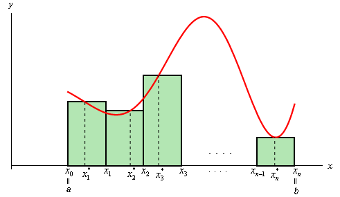
The area under the curve on the given interval is then approximately,

\[A \approx f\left( {x_1^*} \right)\Delta x + f\left( {x_2^*} \right)\Delta x + \cdots + f\left( {x_i^*} \right)\Delta x + \cdots + f\left( {x_n^*} \right)\Delta x\]

We will use summation notation or sigma notation at this point to simplify up our notation a little. If you need a refresher on summation notation check out the section devoted to this in the Extras chapter.

Using summation notation the area estimation is,

\[A \approx \sum\limits_{i = 1}^n {f\left( {x_i^*} \right)\Delta x} \]

The summation in the above equation is called a Riemann Sum.

To get a better estimation we will take $n$ larger and larger. In fact, if we let $n$ go out to infinity we will get the exact area. In other words,

\[A = \mathop {\lim }\limits_{n \to \infty } \sum\limits_{i = 1}^n {f\left( {x_i^*} \right)\Delta x} \]

Before leaving this section let’s address one more issue. To this point we’ve required the function to be positive in our work. Many functions are not positive however. Consider the case of $f\left( x \right) = {x^2} - 4$ on [0,2]. If we use $n = 8$ and the midpoints for the rectangle height we get the following graph,

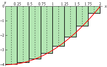
$This is the graph of $f\left( x \right)={{x}^{2}}-4$ on the domain 0<x<2 with 8 rectangles all using the midpoint for the height of the rectangles. Because the graph is completely in the 4th quadrant all of the rectangle go down from the x-axis to the graph of the function.$

In this case let’s notice that the function lies completely below the $x$-axis and hence is always negative. If we ignore the fact that the function is always negative and use the same ideas above to estimate the area between the graph and the $x$-axis we get,

\[\begin{align*}{A_{\,m}} & = \frac{1}{4}f\left( {\frac{1}{8}} \right) + \frac{1}{4}f\left( {\frac{3}{8}} \right) + \frac{1}{4}f\left( {\frac{5}{8}} \right) + \frac{1}{4}f\left( {\frac{7}{8}} \right) + \frac{1}{4}f\left( {\frac{9}{8}} \right) + \\ & \hspace{1.5in}\frac{1}{4}f\left( {\frac{{11}}{8}} \right) + \frac{1}{4}f\left( {\frac{{13}}{8}} \right) + \frac{1}{4}f\left( {\frac{{15}}{8}} \right)\\ & = - 5.34375\end{align*}\]

Our answer is negative as we might have expected given that all the function evaluations are negative.

So, using the technique in this section it looks like if the function is above the $x$-axis we will get a positive area and if the function is below the $x$-axis we will get a negative area. Now, what about a function that is both positive and negative in the interval? For example, $f\left( x \right) = {x^2} - 2$ on [0,2]. Using $n = 8$ and midpoints the graph is,

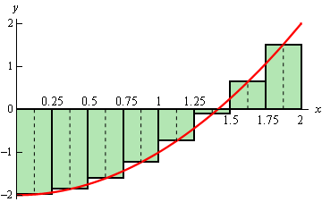
$This is the graph of $f\left( x \right)={{x}^{2}}-2$ on the domain 0<x<2 with 8 rectangles all using the midpoint for the height of the rectangles. The graph starts out below the x-axis and crosses at approximately (1.414,0) and finishes above the x-axis. Because of this the 6 left most rectangles are all below the x-axis and the 2 right most rectangles are both above the x-axis.$

Some of the rectangles are below the $x$-axis and so will give negative areas while some are above the $x$-axis and will give positive areas. Since more rectangles are below the $x$-axis than above it looks like we should probably get a negative area estimation for this case. In fact that is correct. Here the area estimation for this case.

In cases where the function is both above and below the $x$-axis the technique given in the section will give the net area between the function and the $x$-axis with areas below the $x$-axis negative and areas above the $x$-axis positive. So, if the net area is negative then there is more area under the $x$-axis than above while a positive net area will mean that more of the area is above the $x$-axis.