Section 10.13 : Estimating the Value of a Series
We have now spent quite a few sections determining the convergence of a series, however, with the exception of geometric and telescoping series, we have not talked about finding the value of a series. This is usually a very difficult thing to do and we still aren’t going to talk about how to find the value of a series. What we will do is talk about how to estimate the value of a series. Often that is all that you need to know.
Before we get into how to estimate the value of a series let’s remind ourselves how series convergence works. It doesn’t make any sense to talk about the value of a series that doesn’t converge and so we will be assuming that the series we’re working with converges. Also, as we’ll see the main method of estimating the value of series will come out of this discussion.
So, let’s start with the series\(\sum\limits_{n = 1}^\infty {{a_n}} \) (the starting point is not important, but we need a starting point to do the work) and let’s suppose that the series converges to \(s\). Recall that this means that if we get the partial sums,
\[{s_n} = \sum\limits_{i = 1}^n {{a_i}} \]then they will form a convergent sequence and its limit is \(s\). In other words,
\[\mathop {\lim }\limits_{n \to \infty } {s_n} = s\]Now, just what does this mean for us? Well, since this limit converges it means that we can make the partial sums, \({s_n}\), as close to \(s\) as we want simply by taking \(n\) large enough. In other words, if we take \(n\) large enough then we can say that,
\[{s_n} \approx s\]This is one method of estimating the value of a series. We can just take a partial sum and use that as an estimation of the value of the series. There are now two questions that we should ask about this.
First, how good is the estimation? If we don’t have an idea of how good the estimation is then it really doesn’t do all that much for us as an estimation.
Secondly, is there any way to make the estimate better? Sometimes we can use this as a starting point and make the estimation better. We won’t always be able to do this, but if we can that will be nice.
So, let’s start with a general discussion about the determining how good the estimation is. Let’s first start with the full series and strip out the first \(n\) terms.
\[\begin{equation}\sum\limits_{i = 1}^\infty {{a_i}} = \sum\limits_{i = 1}^n {{a_i}} + \sum\limits_{i = n + 1}^\infty {{a_i}} \label{eq:eq1}\end{equation}\]Note that we converted over to an index of \(i\) in order to make the notation consistent with prior notation. Recall that we can use any letter for the index and it won’t change the value.
Now, notice that the first series (the \(n\) terms that we’ve stripped out) is nothing more than the partial sum \({s_n}\). The second series on the right (the one starting at \(i = n + 1\)) is called the remainder and denoted by \({R_n}\). Finally let’s acknowledge that we also know the value of the series since we are assuming it’s convergent. Taking this notation into account we can rewrite \(\eqref{eq:eq1}\) as,
\[s = {s_n} + {R_n}\]We can solve this for the remainder to get,
\[{R_n} = s - {s_n}\]So, the remainder tells us the difference, or error, between the exact value of the series and the value of the partial sum that we are using as the estimation of the value of the series.
Of course, we can’t get our hands on the actual value of the remainder because we don’t have the actual value of the series. However, we can use some of the tests that we’ve got for convergence to get a pretty good estimate of the remainder provided we make some assumptions about the series. Once we’ve got an estimate on the value of the remainder we’ll also have an idea on just how good a job the partial sum does of estimating the actual value of the series.
There are several tests that will allow us to get estimates of the remainder. We’ll go through each one separately.
Also, when using the tests many of them had preconditions for use (i.e. terms had to be positive, terms had to be decreasing etc.) and when using the tests we noted that all we really needed was for them to eventually meet the preconditions in order for the test to work. For the following work however, we need the preconditions to always be met for all terms in the series.
If there are a few terms at the start where the preconditions aren’t met we’ll need to strip those terms out, do the estimate on the series that is left and then add in the terms we stripped out to get a final estimate of the series value.
Integral Test
Recall that in this case we will need to assume that the series terms are all positive and be decreasing for all \(n\). We derived the integral test by using the fact that the series could be thought of as an estimation of the area under the curve of \(f\left( x \right)\) where \(f\left( n \right) = {a_n}\). We can do something similar with the remainder.
As we’ll soon see if we can get an upper and lower bound on the value of the remainder we can use these bounds to help us get upper and lower bounds on the value of the series. We can in turn use the upper and lower bounds on the series value to actually estimate the value of the series.
So, let’s first recall that the remainder is,
\[{R_n} = \sum\limits_{i = n + 1}^\infty {{a_i}} = {a_{n + 1}} + {a_{n + 2}} + {a_{n + 3}} + {a_{n + 4}} + \cdots \]Now, if we start at \(x = n + 1\), take rectangles of width 1 and use the left endpoint as the height of the rectangle we can estimate the area under \(f\left( x \right)\) on the interval \(\left[ {n + 1,\infty } \right)\) as shown in the sketch below.
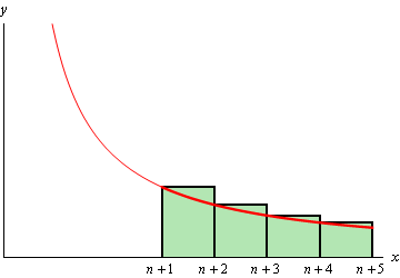
We can see that the remainder, \({R_n}\), is the area estimation and it will overestimate the exact area. So, we have the following inequality.
\[\begin{equation}{R_n} \ge \int_{{\,n + 1}}^{{\,\infty }}{{f\left( x \right)\,dx}}\label{eq:eq2}\end{equation}\]Next, we could also estimate the area by starting at \(x = n\), taking rectangles of width 1 again and then using the right endpoint as the height of the rectangle. This will give an estimation of the area under \(f\left( x \right)\) on the interval \(\left[ {n,\infty } \right)\). This is shown in the following sketch.
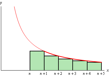
Again, we can see that the remainder, \({R_n}\), is again this estimation and in this case it will underestimate the area. This leads to the following inequality,
\[\begin{equation}{R_n} \le \int_{{\,n}}^{{\,\infty }}{{f\left( x \right)\,dx}}\label{eq:eq3}\end{equation}\]Combining \(\eqref{eq:eq2}\) and \(\eqref{eq:eq3}\) gives,
\[\int_{{\,n + 1}}^{{\,\infty }}{{f\left( x \right)\,dx}} \le {R_n} \le \int_{{\,n}}^{{\,\infty }}{{f\left( x \right)\,dx}}\]So, provided we can do these integrals we can get both an upper and lower bound on the remainder. This will in turn give us an upper bound and a lower bound on just how good the partial sum, \({s_n}\), is as an estimation of the actual value of the series.
In this case we can also use these results to get a better estimate for the actual value of the series as well.
First, we’ll start with the fact that
\[s = {s_n} + {R_n}\]Now, if we use \(\eqref{eq:eq2}\) we get,
\[s = {s_n} + {R_n} \ge {s_n} + \int_{{\,n + 1}}^{{\,\infty }}{{f\left( x \right)\,dx}}\]Likewise if we use \(\eqref{eq:eq3}\) we get,
\[s = {s_n} + {R_n} \le {s_n} + \int_{{\,n}}^{{\,\infty }}{{f\left( x \right)\,dx}}\]Putting these two together gives us,
This gives an upper and a lower bound on the actual value of the series. We could then use as an estimate of the actual value of the series the average of the upper and lower bound.
Let’s work an example with this.
First, for comparison purposes, we’ll note that the actual value of this series is known to be,
\[\sum\limits_{n = 1}^\infty {\frac{1}{{{n^2}}}} = \frac{{{\pi ^2}}}{6} = 1.644934068\]Using \(n = 15\) let’s first get the partial sum.
\[{s_{15}} = \sum\limits_{i = 1}^{15} {\frac{1}{{{i^2}}}} = 1.580440283\]Note that this is “close” to the actual value in some sense but isn’t really all that close either.
Now, let’s compute the integrals. These are fairly simple integrals, so we’ll leave it to you to verify the values.
\[\int_{{\,15}}^{{\,\infty }}{{\frac{1}{{{x^2}}}\,dx}} = \frac{1}{{15}}\hspace{0.25in}\hspace{0.25in}\hspace{0.25in}\int_{{\,16}}^{{\,\infty }}{{\frac{1}{{{x^2}}}\,dx}} = \frac{1}{{16}}\]Plugging these into \(\eqref{eq:eq4}\) gives us,
\[\begin{align*}1.580440283 + \frac{1}{{16}} \le & s \le 1.580440283 + \frac{1}{{15}}\\ 1.642940283 \le & s \le 1.647106950\end{align*}\]Both the upper and lower bound are now very close to the actual value and if we take the average of the two we get the following estimate of the actual value.
\[s \approx 1.6450236165\]That is pretty darn close to the actual value.
So, that is how we can use the Integral Test to estimate the value of a series. Let’s move on to the next test.
Comparison Test
In this case, unlike with the integral test, we may or may not be able to get an idea of how good a particular partial sum will be as an estimate of the exact value of the series. Much of this will depend on how the comparison test is used.
First, let’s remind ourselves on how the comparison test actually works. Given a series \(\sum {{a_n}} \) let’s assume that we’ve used the comparison test to show that it’s convergent. Therefore, we found a second series \(\sum {{b_n}} \) that converged and \({a_n} \le {b_n}\) for all \(n\). Also recall that we need both \({a_n}\) and \({b_n}\) to be positive for all \(n\).
What we want to do is determine how good of a job the partial sum,
\[{s_n} = \sum\limits_{i = 1}^n {{a_i}} \]will do in estimating the actual value of the series \(\sum {{a_n}} \). Again, we will use the remainder to do this. Let’s actually write down the remainder for both series.
\[{R_n} = \sum\limits_{i = n + 1}^\infty {{a_i}} \hspace{0.25in}\hspace{0.25in}\hspace{0.25in}{T_n} = \sum\limits_{i = n + 1}^\infty {{b_i}} \]Now, since \({a_n} \le {b_n}\) we also know that
\[{R_n} \le {T_n}\]When using the comparison test it is often the case that the \({b_n}\) are fairly nice terms and that we might actually be able to get an idea on the size of \({T_n}\). For instance, if our second series is a \(p\)-series we can use the results from above to get an upper bound on \({T_n}\) as follows,
Also, if the second series is a geometric series then we will be able to compute \({T_n}\) exactly.
If we are unable to get an idea of the size of \({T_n}\) then using the comparison test to help with estimates won’t do us much good.
Let’s take a look at an example.
To do this we’ll first need to go through the comparison test so we can get the second series. So,
\[\frac{{{2^n}}}{{{4^n} + 1}} \le \frac{{{2^n}}}{{{4^n}}} = {\left( {\frac{1}{2}} \right)^n}\]and
\[\sum\limits_{n = 0}^\infty {{{\left( {\frac{1}{2}} \right)}^n}} \]is a geometric series and converges because \(\left| r \right| = \frac{1}{2} < 1\).
Now that we’ve gotten our second series let’s get the estimate.
\[{s_{15}} = \sum\limits_{n = 0}^{15} {\frac{{{2^n}}}{{{4^n} + 1}}} = 1.383062486\]So, how good is it? Well we know that,
\[{R_{15}} \le {T_{15}} = \sum\limits_{n = 16}^\infty {{{\left( {\frac{1}{2}} \right)}^n}} \]will be an upper bound for the error between the actual value and the estimate. Since our second series is a geometric series we can compute this directly as follows.
\[\sum\limits_{n = 0}^\infty {{{\left( {\frac{1}{2}} \right)}^n}} = \sum\limits_{n = 0}^{15} {{{\left( {\frac{1}{2}} \right)}^n}} + \sum\limits_{n = 16}^\infty {{{\left( {\frac{1}{2}} \right)}^n}} \]The series on the left is in the standard form and so we can compute that directly. The first series on the right has a finite number of terms and so can be computed exactly and the second series on the right is the one that we’d like to have the value for. Doing the work gives,
\[\begin{align*}\sum\limits_{n = 16}^\infty {{{\left( {\frac{1}{2}} \right)}^n}} & = \sum\limits_{n = 0}^\infty {{{\left( {\frac{1}{2}} \right)}^n}} - \sum\limits_{n = 0}^{15} {{{\left( {\frac{1}{2}} \right)}^n}} \\ & = \frac{1}{{1 - \left( {\frac{1}{2}} \right)}} - 1.999969482\\ & = 0.000030518\end{align*}\]So, according to this if we use
\[s \approx 1.383062486\]as an estimate of the actual value we will be off from the exact value by no more than \(0.000030518\) and that’s not too bad.
In this case it can be shown that
\[\sum\limits_{n = 0}^\infty {\frac{{{2^n}}}{{{4^n} + 1}}} = 1.383093004\]and so we can see that the actual error in our estimation is,
\[{\mbox{Error}} = {\mbox{Actual}} - {\mbox{Estimate}} = 1.383093004 - 1.383062486 = 0.000030518\]Note that in this case the estimate of the error is actually fairly close (and in fact exactly the same) as the actual error. This will not always happen and so we shouldn’t expect that to happen in all cases. The error estimate above is simply the upper bound on the error and the actual error will often be less than this value.
Before moving on to the final part of this section let’s again note that we will only be able to determine how good the estimate is using the comparison test if we can easily get our hands on the remainder of the second term. The reality is that we won’t always be able to do this.
Alternating Series Test
Both of the methods that we’ve looked at so far have required the series to contain only positive terms. If we allow series to have negative terms in it the process is usually more difficult. However, with that said there is one case where it isn’t too bad. That is the case of an alternating series.
Once again we will start off with a convergent series \(\sum {{a_n} = \sum {{{\left( { - 1} \right)}^n}{b_n}} } \) which in this case happens to be an alternating series that satisfies the conditions of the alternating series test, so we know that \({b_n} \ge 0\) and is decreasing for all \(n\). Also note that we could have any power on the “-1” we just used \(n\) for the sake of convenience. We want to know how good of an estimation of the actual series value will the partial sum, \({s_n}\), be. As with the prior cases we know that the remainder, \({R_n}\), will be the error in the estimation and so if we can get a handle on that we’ll know approximately how good the estimation is.
From the proof of the Alternating Series Test we can see that \(s\) will lie between \({s_n}\) and \({s_{n + 1}}\) for any \(n\) and so,
\[\left| {s - {s_n}} \right| \le \left| {{s_{n + 1}} - {s_n}} \right| = {b_{n + 1}}\]Therefore,
We needed absolute value bars because we won’t know ahead of time if the estimation is larger or smaller than the actual value and we know that the \({b_n}\)’s are positive.
Let’s take a look at an example.
This is an alternating series and it does converge. In this case the exact value is known and so for comparison purposes,
\[\sum\limits_{n = 1}^\infty {\frac{{{{\left( { - 1} \right)}^n}}}{{{n^2}}}} = - \frac{{{\pi ^2}}}{{12}} = - 0.8224670336\]Now, the estimation is,
\[{s_{15}} = \sum\limits_{n = 1}^{15} {\frac{{{{\left( { - 1} \right)}^n}}}{{{n^2}}}} = - 0.8245417574\]From the fact above we know that
\[\left| {{R_{15}}} \right| = \left| {s - {s_{15}}} \right| \le {b_{16}} = \frac{1}{{{{16}^2}}} = 0.00390625\]So, our estimation will have an error of no more than 0.00390625. In this case the exact value is known and so the actual error is,
\[\left| {{R_{15}}} \right| = \left| {s - {s_{15}}} \right| = 0.0020747238\]In the previous example the estimation had only half the estimated error. It will often be the case that the actual error will be less than the estimated error. Remember that this is only an upper bound for the actual error.
Ratio Test
This will be the final case that we’re going to look at for estimating series values and we are going to have to put a couple of fairly stringent restrictions on the series terms in order to do the work. One of the main restrictions we’re going to make is to assume that the series terms are positive even though that is not required to actually use the test. We’ll also be adding on another restriction in a bit.
In this case we’ve used the ratio test to show that \(\sum {{a_n}} \) is convergent. To do this we computed
\[L = \mathop {\lim }\limits_{n \to \infty } \left| {\frac{{{a_{n + 1}}}}{{{a_n}}}} \right|\]and found that \(L < 1\).
As with the previous cases we are going to use the remainder, \({R_n}\), to determine how good of an estimation of the actual value the partial sum, \({s_n}\), is.
To get an estimate of the remainder let’s first define the following sequence,
\[{r_n} = \frac{{{a_{n + 1}}}}{{{a_n}}}\]We now have two possible cases.
- If \(\left\{ {{r_{n}}} \right\}\) is a decreasing sequence and \({r_{n + 1}} < 1\) then, \[{R_n} \le \frac{{{a_{n + 1}}}}{{1 - {r_{n + 1}}}}\]
- If \(\left\{ {{r_{n}}} \right\}\) is an increasing sequence then, \[{R_n} \le \frac{{{a_{n + 1}}}}{{1 - L}}\]
Proof
Both parts will need the following work so we’ll do it first. We’ll start with the remainder.
\[\begin{align*}{R_n} = \sum\limits_{i = n + 1}^\infty {{a_i}} & = {a_{n + 1}} + {a_{n + 2}} + {a_{n + 3}} + {a_{n + 4}} + \cdots \\ & = {a_{n + 1}}\left( {1 + \frac{{{a_{n + 2}}}}{{{a_{n + 1}}}} + \frac{{{a_{n + 3}}}}{{{a_{n + 1}}}} + \frac{{{a_{n + 4}}}}{{{a_{n + 1}}}} + \cdots } \right)\end{align*}\]Next, we need to do a little work on a couple of these terms.
\[\begin{align*}{R_n} & = {a_{n + 1}}\left( {1 + \frac{{{a_{n + 2}}}}{{{a_{n + 1}}}} + \frac{{{a_{n + 3}}}}{{{a_{n + 1}}}}\frac{{{a_{n + 2}}}}{{{a_{n + 2}}}} + \frac{{{a_{n + 4}}}}{{{a_{n + 1}}}}\frac{{{a_{n + 2}}}}{{{a_{n + 2}}}}\frac{{{a_{n + 3}}}}{{{a_{n + 3}}}} + \cdots } \right)\\ & = {a_{n + 1}}\left( {1 + \frac{{{a_{n + 2}}}}{{{a_{n + 1}}}} + \frac{{{a_{n + 2}}}}{{{a_{n + 1}}}}\frac{{{a_{n + 3}}}}{{{a_{n + 2}}}} + \frac{{{a_{n + 2}}}}{{{a_{n + 1}}}}\frac{{{a_{n + 3}}}}{{{a_{n + 2}}}}\frac{{{a_{n + 4}}}}{{{a_{n + 3}}}} + \cdots } \right)\end{align*}\]Now use the definition of \({r_n}\) to write this as,
\[{R_n} = {a_{n + 1}}\left( {1 + {r_{n + 1}} + {r_{n + 1}}{r_{n + 2}} + {r_{n + 1}}{r_{n + 2}}{r_{n + 3}} + \cdots } \right)\]Okay now let’s do the proof.
For the first part we are assuming that \(\left\{ {{r_{n}}} \right\}\) is decreasing and so we can estimate the remainder as,
\[\begin{align*}{R_n} & = {a_{n + 1}}\left( {1 + {r_{n + 1}} + {r_{n + 1}}{r_{n + 2}} + {r_{n + 1}}{r_{n + 2}}{r_{n + 3}} + \cdots } \right)\\ & \le {a_{n + 1}}\left( {1 + {r_{n + 1}} + r_{n + 1}^2 + r_{n + 1}^3 + \cdots } \right)\\ & = {a_{n + 1}}\sum\limits_{k = 0}^\infty {r_{n + 1}^k} \end{align*}\]Finally, the series here is a geometric series and because \({r_{n + 1}} < 1\) we know that it converges and we can compute its value. So,
\[{R_n} \le \frac{{{a_{n + 1}}}}{{1 - {r_{n + 1}}}}\]For the second part we are assuming that \(\left\{ {{r_{n}}} \right\}\) is increasing and we know that,
\[\mathop {\lim }\limits_{n \to \infty } \left| {{r_n}} \right| = \mathop {\lim }\limits_{n \to \infty } \left| {\frac{{{a_{n + 1}}}}{{{a_n}}}} \right| = L\]and so we know that \({r_n} < L\) for all \(n\). The remainder can then be estimated as,
\[\begin{align*}{R_n} & = {a_{n + 1}}\left( {1 + {r_{n + 1}} + {r_{n + 1}}{r_{n + 2}} + {r_{n + 1}}{r_{n + 2}}{r_{n + 3}} + \cdots } \right)\\ & \le {a_{n + 1}}\left( {1 + L + {L^2} + {L^3} + \cdots } \right)\\ & = {a_{n + 1}}\sum\limits_{k = 0}^\infty {{L^k}} \end{align*}\]This is a geometric series and since we are assuming that our original series converges we also know that \(L < 1\) and so the geometric series above converges and we can compute its value. So,
\[{R_n} \le \frac{{{a_{n + 1}}}}{{1 - L}}\]Note that there are some restrictions on the sequence \(\left\{ {{r_{n}}} \right\}\) and at least one of its terms in order to use these formulas. If the restrictions aren’t met then the formulas can’t be used.
Let’s take a look at an example of this.
First, let’s use the ratio test to verify that this is a convergent series.
\[L = \mathop {\lim }\limits_{n \to \infty } \left| {\frac{{n + 1}}{{{3^{n + 1}}}}\,\,\frac{{{3^n}}}{n}} \right| = \mathop {\lim }\limits_{n \to \infty } \frac{{n + 1}}{{3n}} = \frac{1}{3} < 1\]So, it is convergent. Now let’s get the estimate.
\[{s_{15}} = \sum\limits_{n = 0}^{15} {\frac{n}{{{3^n}}}} = 0.7499994250\]To determine an estimate on the remainder, and hence the error, let’s first get the sequence \(\left\{ {{r_{n}}} \right\}\).
\[{r_n} = \frac{{n + 1}}{{{3^{n + 1}}}}\,\,\frac{{{3^n}}}{n} = \frac{{n + 1}}{{3n}} = \frac{1}{3}\left( {1 + \frac{1}{n}} \right)\]The last rewrite was just to simplify some of the computations a little. Now, notice that,
\[f\left( x \right) = \frac{1}{3}\left( {1 + \frac{1}{x}} \right)\hspace{0.25in}\hspace{0.25in}f'\left( x \right) = - \frac{1}{{3{x^2}}} < 0\]Since this function is always decreasing and \(f\left( n \right) = {r_n}\) this sequence is decreasing. Also note that \({r_{16}} = \frac{1}{3}\left( {1 + \frac{1}{{16}}} \right) < 1\). Therefore, we can use the first case from the fact above to get,
\[{R_{15}} \le \frac{{{a_{16}}}}{{1 - {r_{16}}}} = \frac{{\frac{{16}}{{{3^{16}}}}}}{{1 - \frac{1}{3}\left( {1 + \frac{1}{{16}}} \right)}} = 0.0000005755187\]So, it looks like our estimate is probably quite good. In this case the exact value is known.
\[\sum\limits_{n = 0}^\infty {\frac{n}{{{3^n}}}} = \frac{3}{4}\]and so we can compute the actual error.
\[\left| {{R_{15}}} \right| = \left| {s - {s_{15}}} \right| = 0.000000575\]This is less than the upper bound, but unlike in the previous example this actual error is quite close to the upper bound.
In the last two examples we’ve seen that the upper bound computations on the error can sometimes be quite close to the actual error and at other times they can be off by quite a bit. There is usually no way of knowing ahead of time which it will be and without the exact value in hand there will never be a way of determining which it will be.
Notice that this method did require the series terms to be positive, but that doesn’t mean that we can’t deal with ratio test series if they have negative terms. Often series that we used ratio test on are also alternating series and so if that is the case we can always resort to the previous material to get an upper bound on the error in the estimation, even if we didn’t use the alternating series test to show convergence.
Note however that if the series does have negative terms but doesn’t happen to be an alternating series then we can’t use any of the methods discussed in this section to get an upper bound on the error.