Section 14.3 : Relative Minimums and Maximums
In this section we are going to extend one of the more important ideas from Calculus I into functions of two variables. We are going to start looking at trying to find minimums and maximums of functions. This in fact will be the topic of the following two sections as well.
In this section we are going to be looking at identifying relative minimums and relative maximums. Recall as well that we will often use the word extrema to refer to both minimums and maximums.
The definition of relative extrema for functions of two variables is identical to that for functions of one variable we just need to remember now that we are working with functions of two variables. So, for the sake of completeness here is the definition of relative minimums and relative maximums for functions of two variables.
Definition
- A function \(f\left( {x,y} \right)\) has a relative minimum at the point \(\left( {a,b} \right)\) if \(f\left( {x,y} \right) \ge f\left( {a,b} \right)\) for all points\(\left( {x,y} \right)\) in some region around \(\left( {a,b} \right)\).
- A function \(f\left( {x,y} \right)\) has a relative maximum at the point \(\left( {a,b} \right)\) if \(f\left( {x,y} \right) \le f\left( {a,b} \right)\) for all points\(\left( {x,y} \right)\) in some region around \(\left( {a,b} \right)\).
Note that this definition does not say that a relative minimum is the smallest value that the function will ever take. It only says that in some region around the point \(\left( {a,b} \right)\) the function will always be larger than \(f\left( {a,b} \right)\). Outside of that region it is completely possible for the function to be smaller. Likewise, a relative maximum only says that around \(\left( {a,b} \right)\) the function will always be smaller than \(f\left( {a,b} \right)\). Again, outside of the region it is completely possible that the function will be larger.
Next, we need to extend the idea of critical points up to functions of two variables. Recall that a critical point of the function \(f\left( x \right)\) was a number \(x = c\) so that either \(f'\left( c \right) = 0\) or \(f'\left( c \right)\) doesn’t exist. We have a similar definition for critical points of functions of two variables.
Definition
The point \(\left( {a,b} \right)\) is a critical point (or a stationary point) of \(f\left( {x,y} \right)\) provided one of the following is true,
- \(\nabla f\left( {a,b} \right) = \vec 0\) (this is equivalent to saying that \({f_x}\left( {a,b} \right) = 0\) and \({f_y}\left( {a,b} \right) = 0\)),
- \({f_x}\left( {a,b} \right)\) and/or \({f_y}\left( {a,b} \right)\) doesn’t exist.
To see the equivalence in the first part let’s start off with \(\nabla f = \vec 0\) and put in the definition of each part.
\[\begin{align*}\nabla f\left( {a,b} \right) & = \vec 0\\ \left\langle {{f_x}\left( {a,b} \right),{f_y}\left( {a,b} \right)} \right\rangle & = \left\langle {0,0} \right\rangle \end{align*}\]The only way that these two vectors can be equal is to have \({f_x}\left( {a,b} \right) = 0\) and \({f_y}\left( {a,b} \right) = 0\). In fact, we will use this definition of the critical point more than the gradient definition since it will be easier to find the critical points if we start with the partial derivative definition.
Note as well that BOTH of the first order partial derivatives must be zero at \(\left( {a,b} \right)\). If only one of the first order partial derivatives are zero at the point then the point will NOT be a critical point.
We now have the following fact that, at least partially, relates critical points to relative extrema.
Fact
If the point \(\left( {a,b} \right)\) is a relative extrema of the function \(f\left( {x,y} \right)\) and the first order derivatives of \(f\left( {x,y} \right)\) exist at \(\left( {a,b} \right)\) then \(\left( {a,b} \right)\) is also a critical point of \(f\left( {x,y} \right)\) and in fact we’ll have \(\nabla f\left( {a,b} \right) = \vec 0\).
Proof
This is a really simple proof that relies on the single variable version that we saw in Calculus I version, often called Fermat’s Theorem.
Let’s start off by defining \(g\left( x \right) = f\left( {x,b} \right)\) and suppose that \(f\left( {x,y} \right)\) has a relative extrema at \(\left( {a,b} \right)\). However, this also means that \(g\left( x \right)\) also has a relative extrema (of the same kind as \(f\left( {x,y} \right)\)) at \(x = a\). By Fermat’s Theorem we then know that \(g'\left( a \right) = 0\). But we also know that \(g'\left( a \right) = {f_x}\left( {a,b} \right)\) and so we have that \({f_x}\left( {a,b} \right) = 0\).
If we now define \(h\left( y \right) = f\left( {a,y} \right)\) and going through exactly the same process as above we will see that \({f_y}\left( {a,b} \right) = 0\).
So, putting all this together means that \(\nabla f\left( {a,b} \right) = \vec 0\) and so \(f\left( {x,y} \right)\) has a critical point at \(\left( {a,b} \right)\).
Note that this does NOT say that all critical points are relative extrema. It only says that relative extrema will be critical points of the function. To see this let’s consider the function
\[f\left( {x,y} \right) = xy\]The two first order partial derivatives are,
\[{f_x}\left( {x,y} \right) = y\hspace{0.75in}{f_y}\left( {x,y} \right) = x\]The only point that will make both of these derivatives zero at the same time is \(\left( {0,0} \right)\) and so \(\left( {0,0} \right)\) is a critical point for the function. Here is a graph of the function.
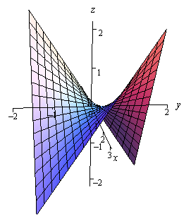
Note that the axes are not in the standard orientation here so that we can see more clearly what is happening at the origin, i.e. at \(\left( {0,0} \right)\). If we start at the origin and move into either of the quadrants where both \(x\) and \(y\) are the same sign the function increases. However, if we start at the origin and move into either of the quadrants where \(x\) and \(y\) have the opposite sign then the function decreases. In other words, no matter what region you take about the origin there will be points larger than \(f\left( {0,0} \right) = 0\) and points smaller than \(f\left( {0,0} \right) = 0\). Therefore, there is no way that \(\left( {0,0} \right)\) can be a relative extrema.
Critical points that exhibit this kind of behavior are called saddle points.
While we have to be careful to not misinterpret the results of this fact it is very useful in helping us to identify relative extrema. Because of this fact we know that if we have all the critical points of a function then we also have every possible relative extrema for the function. The fact tells us that all relative extrema must be critical points so we know that if the function does have relative extrema then they must be in the collection of all the critical points. Remember however, that it will be completely possible that at least one of the critical points won’t be a relative extrema.
So, once we have all the critical points in hand all we will need to do is test these points to see if they are relative extrema or not. To determine if a critical point is a relative extrema (and in fact to determine if it is a minimum or a maximum) we can use the following fact.
Fact
Suppose that \(\left( {a,b} \right)\) is a critical point of \(f\left( {x,y} \right)\) and that the second order partial derivatives are continuous in some region that contains \(\left( {a,b} \right)\). Next define,
\[D = D\left( {a,b} \right) = {f_{x\,x}}\left( {a,b} \right){f_{y\,y}}\left( {a,b} \right) - {\left[ {{f_{x\,y}}\left( {a,b} \right)} \right]^2}\]We then have the following classifications of the critical point.
- If \(D > 0\) and \({f_{x\,x}}\left( {a,b} \right) > 0\) then there is a relative minimum at \(\left( {a,b} \right)\).
- If \(D > 0\) and \({f_{x\,x}}\left( {a,b} \right) < 0\) then there is a relative maximum at \(\left( {a,b} \right)\).
- If \(D < 0\) then the point \(\left( {a,b} \right)\) is a saddle point.
- If \(D = 0\) then the point \(\left( {a,b} \right)\) may be a relative minimum, relative maximum or a saddle point. Other techniques would need to be used to classify the critical point.
Note that if \(D > 0\) then both \({f_{\,x\,x}}\left( {a,b} \right)\) and \({f_{\,y\,y}}\left( {a,b} \right)\) will have the same sign and so in the first two cases above we could just as easily replace \({f_{\,x\,x}}\left( {a,b} \right)\) with \({f_{\,y\,y}}\left( {a,b} \right)\). Also note that we aren’t going to be seeing any cases in this class where \(D = 0\) as these can often be quite difficult to classify. We will be able to classify all the critical points that we find.
Let’s see a couple of examples.
We first need all the first order (to find the critical points) and second order (to classify the critical points) partial derivatives so let’s get those.
\[\begin{array}{c}{f_x} = 3{x^2} - 3y\hspace{0.5in}{f_y} = 3{y^2} - 3x\\ {f_{x\,x}} = 6x\hspace{0.5in}{f_{y\,y}} = 6y\hspace{0.5in}{f_{x\,y}} = - 3\end{array}\]Let’s first find the critical points. Critical points will be solutions to the system of equations,
\[\begin{align*}{f_x} & = 3{x^2} - 3y = 0\\ {f_y} & = 3{y^2} - 3x = 0\end{align*}\]This is a non-linear system of equations and these can, on occasion, be difficult to solve. However, in this case it’s not too bad. We can solve the first equation for \(y\) as follows,
\[3{x^2} - 3y = 0\hspace{0.25in} \Rightarrow \hspace{0.25in}y = {x^2}\]Plugging this into the second equation gives,
\[3{\left( {{x^2}} \right)^2} - 3x = 3x\left( {{x^3} - 1} \right) = 0\]From this we can see that we must have \(x = 0\) or \(x = 1\). Now use the fact that \(y = {x^2}\) to get the critical points.
\[\begin{align*}x = 0: & \hspace{0.25in}y = {0^2} = 0\hspace{0.1in} & \Rightarrow & \hspace{0.5in}\left( {0,0} \right)\\ x = 1: & \hspace{0.25in}y = {1^2} = 1\hspace{0.1in} & \Rightarrow & \hspace{0.5in}\left( {1,1} \right)\end{align*}\]So, we get two critical points. All we need to do now is classify them. To do this we will need \(D\). Here is the general formula for \(D\).
\[\begin{align*}D\left( {x,y} \right) & = {f_{x\,x}}\left( {x,y} \right){f_{y\,y}}\left( {x,y} \right) - {\left[ {{f_{x\,y}}\left( {x,y} \right)} \right]^2}\\ & = \left( {6x} \right)\left( {6y} \right) - {\left( { - 3} \right)^2}\\ & = 36xy - 9\end{align*}\]To classify the critical points all that we need to do is plug in the critical points and use the fact above to classify them.
\(\left( {0,0} \right)\) : \[D = D\left( {0,0} \right) = - 9 < 0\]So, for \(\left( {0,0} \right)\) \(D\) is negative and so this must be a saddle point.
\(\left( {1,1} \right)\) : \[D = D\left( {1,1} \right) = 36 - 9 = 27 > 0\hspace{0.5in}{f_{x\,x}}\left( {1,1} \right) = 6 > 0\]For \(\left( {1,1} \right)\) \(D\) is positive and \({f_{x\,x}}\) is positive and so we must have a relative minimum.
For the sake of completeness here is a graph of this function.
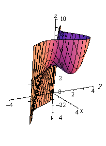
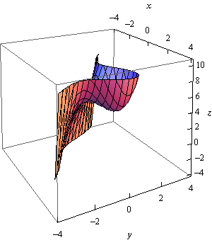
Notice that in order to get a better visual we used a somewhat nonstandard orientation. We can see that there is a relative minimum at \(\left( {1,1} \right)\) and (hopefully) it’s clear that at \(\left( {0,0} \right)\) we do get a saddle point.
As with the first example we will first need to get all the first and second order derivatives.
\[\begin{array}{c}{f_x} = 6xy - 6x\hspace{0.5in}{f_y} = 3{x^2} + 3{y^2} - 6y\\ {f_{x\,x}} = 6y - 6\hspace{0.5in}{f_{y\,y}} = 6y - 6\hspace{0.75in}{f_{x\,y}} = 6x\end{array}\]We’ll first need the critical points. The equations that we’ll need to solve this time are,
\[\begin{align*}6xy - 6x & = 0\\ 3{x^2} + 3{y^2} - 6y & = 0\end{align*}\]These equations are a little trickier to solve than the first set, but once you see what to do they really aren’t terribly bad.
First, let’s notice that we can factor out a 6\(x\) from the first equation to get,
\[6x\left( {y - 1} \right) = 0\]So, we can see that the first equation will be zero if \(x = 0\) or \(y = 1\). Be careful to not just cancel the \(x\) from both sides. If we had done that we would have missed \(x = 0\).
To find the critical points we can plug these (individually) into the second equation and solve for the remaining variable.
\(x = 0\) : \[3{y^2} - 6y = 3y\left( {y - 2} \right) = 0\hspace{0.25in} \Rightarrow \hspace{0.25in}y = 0,\,\,y = 2\] \(y = 1\) : \[3{x^2} - 3 = 3\left( {{x^2} - 1} \right) = 0\hspace{0.5in} \Rightarrow \hspace{0.25in}x = - 1,\,\,x = 1\]So, if \(x = 0\) we have the following critical points,
\[\left( {0,0} \right)\hspace{0.25in}\left( {0,2} \right)\]and if \(y = 1\) the critical points are,
\[\left( {1,1} \right)\hspace{0.25in}\left( { - 1,1} \right)\]Now all we need to do is classify the critical points. To do this we’ll need the general formula for \(D\).
\[D\left( {x,y} \right) = \left( {6y - 6} \right)\left( {6y - 6} \right) - {\left( {6x} \right)^2} = {\left( {6y - 6} \right)^2} - 36{x^2}\] \(\left( {0,0} \right)\) : \[D = D\left( {0,0} \right) = 36 > 0\hspace{0.5in}{f_{x\,x}}\left( {0,0} \right) = - 6 < 0\] \(\left( {0,2} \right)\) : \[D = D\left( {0,2} \right) = 36 > 0\hspace{0.5in}{f_{x\,x}}\left( {0,2} \right) = 6 > 0\] \(\left( {1,1} \right)\) : \[D = D\left( {1,1} \right) = - 36 < 0\] \(\left( { - 1,1} \right)\) : \[D = D\left( { - 1,1} \right) = - 36 < 0\]So, it looks like we have the following classification of each of these critical points.
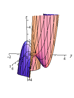
\[\begin{align*} & \left( {0,0} \right) & & :\hspace{0.5in}{\mbox{Relative Maximum}}\\ & \left( {0,2} \right) & & : \hspace{0.5in} {\mbox{Relative Minimum}}\\ & \left( {1,1} \right) & & :\hspace{0.5in}{\mbox{Saddle Point}}\\ & \left( { - 1,1} \right) & & :\hspace{0.5in}{\mbox{Saddle Point}}\end{align*}\]Here is a graph of the surface for the sake of completeness.
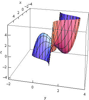
Let’s do one more example that is a little different from the first two.
Note that we are NOT asking for the critical points of the plane. In order to do this example we are going to need to first come up with the equation that we are going to have to work with.
First, let’s suppose that \(\left( {x,y,z} \right)\) is any point on the plane. The distance between this point and the point in question, \(\left( { - 2, - 1,5} \right)\), is given by the formula,
\[d = \sqrt {{{\left( {x + 2} \right)}^2} + {{\left( {y + 1} \right)}^2} + {{\left( {z - 5} \right)}^2}} \]What we are then asked to find is the minimum value of this equation. The point \(\left( {x,y,z} \right)\) that gives the minimum value of this equation will be the point on the plane that is closest to \(\left( { - 2, - 1,5} \right)\).
There are a couple of issues with this equation. First, it is a function of \(x\), \(y\) and \(z\) and we can only deal with functions of \(x\) and \(y\) at this point. However, this is easy to fix. We can solve the equation of the plane to see that,
\[z = 1 - 4x + 2y\]Plugging this into the distance formula gives,
\[\begin{align*}d & = \sqrt {{{\left( {x + 2} \right)}^2} + {{\left( {y + 1} \right)}^2} + {{\left( {1 - 4x + 2y - 5} \right)}^2}} \\ & = \sqrt {{{\left( {x + 2} \right)}^2} + {{\left( {y + 1} \right)}^2} + {{\left( { - 4 - 4x + 2y} \right)}^2}} \end{align*}\]Now, the next issue is that there is a square root in this formula and we know that we’re going to be differentiating this eventually. So, in order to make our life a little easier let’s notice that finding the minimum value of \(d\) will be equivalent to finding the minimum value of \({d^2}\).
So, let’s instead find the minimum value of
\[f\left( {x,y} \right) = {d^2} = {\left( {x + 2} \right)^2} + {\left( {y + 1} \right)^2} + {\left( { - 4 - 4x + 2y} \right)^2}\]Now, we need to be a little careful here. We are being asked to find the closest point on the plane to \(\left( { - 2, - 1,5} \right)\) and that is not really the same thing as what we’ve been doing in this section. In this section we’ve been finding and classifying critical points as relative minimums or maximums and what we are really asking is to find the smallest value the function will take, or the absolute minimum. Hopefully, it does make sense from a physical standpoint that there will be a closest point on the plane to \(\left( { - 2, - 1,5} \right)\). This point should also be a relative minimum in addition to being an absolute minimum.
So, let’s go through the process from the first and second example and see what we get as far as relative minimums go. If we only get a single relative minimum then we will be done since that point will also need to be the absolute minimum of the function and hence the point on the plane that is closest to \(\left( { - 2, - 1,5} \right)\).
We’ll need the derivatives first.
\[\begin{align*}{f_x} & = 2\left( {x + 2} \right) + 2\left( { - 4} \right)\left( { - 4 - 4x + 2y} \right) = 36 + 34x - 16y\\ {f_y} & = 2\left( {y + 1} \right) + 2\left( 2 \right)\left( { - 4 - 4x + 2y} \right) = - 14 - 16x + 10y\\ {f_{x\,x}} & = 34\\ {f_{y\,y}} & = 10\\ {f_{x\,y}} & = - 16\end{align*}\]Now, before we get into finding the critical point let’s compute \(D\) quickly.
\[D = 34\left( {10} \right) - {\left( { - 16} \right)^2} = 84 > 0\]So, in this case \(D\) will always be positive and also notice that \({f_{x\,x}} = 34 > 0\) is always positive and so any critical points that we get will be guaranteed to be relative minimums.
Now let’s find the critical point(s). This will mean solving the system.
\[\begin{align*}36 + 34x - 16y & = 0\\ - 14 - 16x + 10y & = 0\end{align*}\]To do this we can solve the first equation for \(x\).
\[x = \frac{1}{{34}}\left( {16y - 36} \right) = \frac{1}{{17}}\left( {8y - 18} \right)\]Now, plug this into the second equation and solve for \(y\).
\[ - 14 - \frac{{16}}{{17}}\left( {8y - 18} \right) + 10y = 0\hspace{0.5in} \Rightarrow \hspace{0.5in}y = - \frac{{25}}{{21}}\]Back substituting this into the equation for \(x\) gives \(x = - \frac{{34}}{{21}}\).
So, it looks like we get a single critical point : \(\left( { - \frac{{34}}{{21}}, - \frac{{25}}{{21}}} \right)\). Also, since we know this will be a relative minimum and it is the only critical point we know that this is also the \(x\) and \(y\) coordinates of the point on the plane that we’re after. We can find the \(z\) coordinate by plugging into the equation of the plane as follows,
\[z = 1 - 4\left( { - \frac{{34}}{{21}}} \right) + 2\left( { - \frac{{25}}{{21}}} \right) = \frac{{107}}{{21}}\]So, the point on the plane that is closest to \(\left( { - 2, - 1,5} \right)\) is \(\left( { - \frac{{34}}{{21}}, - \frac{{25}}{{21}},\frac{{107}}{{21}}} \right)\).