Section 9.7 : Laplace's Equation
The next partial differential equation that we’re going to solve is the 2-D Laplace’s equation,
\[{\nabla ^2}u = \frac{{{\partial ^2}u}}{{\partial {x^2}}} + \frac{{{\partial ^2}u}}{{\partial {y^2}}} = 0\]A natural question to ask before we start learning how to solve this is does this equation come up naturally anywhere? The answer is a very resounding yes! If we consider the 2‑D heat equation,
\[\frac{{\partial u}}{{\partial t}} = k{\nabla ^2}u + \frac{Q}{{cp}}\]We can see that Laplace’s equation would correspond to finding the equilibrium solution (i.e. time independent solution) if there were not sources. So, this is an equation that can arise from physical situations.
How we solve Laplace’s equation will depend upon the geometry of the 2-D object we’re solving it on. Let’s start out by solving it on the rectangle given by \(0 \le x \le L\),\(0 \le y \le H\). For this geometry Laplace’s equation along with the four boundary conditions will be,
\[\begin{equation}\begin{aligned}& {\nabla ^2}u = \frac{{{\partial ^2}u}}{{\partial {x^2}}} + \frac{{{\partial ^2}u}}{{\partial {y^2}}} = 0\\ & u\left( {0,y} \right) = {g_1}\left( y \right)\hspace{0.25in}u\left( {L,y} \right) = {g_2}\left( y \right)\\ & u\left( {x,0} \right) = {f_1}\left( x \right)\hspace{0.25in}u\left( {x,H} \right) = {f_2}\left( x \right)\end{aligned}\label{eq:eq1}\end{equation}\]One of the important things to note here is that unlike the heat equation we will not have any initial conditions here. Both variables are spatial variables and each variable occurs in a 2nd order derivative and so we’ll need two boundary conditions for each variable.
Next, let’s notice that while the partial differential equation is both linear and homogeneous the boundary conditions are only linear and are not homogeneous. This creates a problem because separation of variables requires homogeneous boundary conditions.
To completely solve Laplace’s equation we’re in fact going to have to solve it four times. Each time we solve it only one of the four boundary conditions can be nonhomogeneous while the remaining three will be homogeneous.
The four problems are probably best shown with a quick sketch so let’s consider the following sketch.
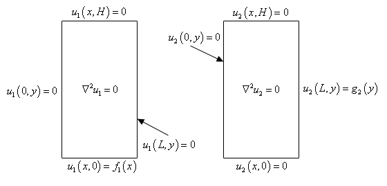
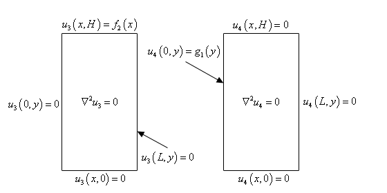
Now, once we solve all four of these problems the solution to our original system, \(\eqref{eq:eq1}\), will be,
\[u\left( {x,y} \right) = {u_1}\left( {x,y} \right) + {u_2}\left( {x,y} \right) + {u_3}\left( {x,y} \right) + {u_4}\left( {x,y} \right)\]Because we know that Laplace’s equation is linear and homogeneous and each of the pieces is a solution to Laplace’s equation then the sum will also be a solution. Also, this will satisfy each of the four original boundary conditions. We’ll verify the first one and leave the rest to you to verify.
\[u\left( {x,0} \right) = {u_1}\left( {x,0} \right) + {u_2}\left( {x,0} \right) + {u_3}\left( {x,0} \right) + {u_4}\left( {x,0} \right) = {f_1}\left( x \right) + 0 + 0 + 0 = {f_1}\left( x \right)\]In each of these cases the lone nonhomogeneous boundary condition will take the place of the initial condition in the heat equation problems that we solved a couple of sections ago. We will apply separation of variables to each problem and find a product solution that will satisfy the differential equation and the three homogeneous boundary conditions. Using the Principle of Superposition we’ll find a solution to the problem and then apply the final boundary condition to determine the value of the constant(s) that are left in the problem. The process is nearly identical in many ways to what we did when we were solving the heat equation.
We’re going to do two of the cases here and we’ll leave the remaining two for you to do.
We’ll start by assuming that our solution will be in the form,
\[{u_4}\left( {x,y} \right) = h\left( x \right)\varphi \left( y \right)\]and then recall that we performed separation of variables on this problem (with a small change in notation) back in Example 5 of the Separation of Variables section. So from that problem we know that separation of variables yields the following two ordinary differential equations that we’ll need to solve.
\[\begin{align*} & \frac{{{d^2}h}}{{d{x^2}}} - \lambda h = 0 & \hspace{0.25in} & \frac{{{d^2} \varphi }}{{d{y^2}}} + \lambda \varphi = 0\\ & h\left( L \right) = 0 & \hspace{0.25in}& \varphi \left( 0 \right) = 0\hspace{0.25in} \varphi \left( H \right) = 0\end{align*}\]Note that in this case, unlike the heat equation we must solve the boundary value problem first. Without knowing what \(\lambda \)is there is no way that we can solve the first differential equation here with only one boundary condition since the sign of \(\lambda \) will affect the solution.
Let’s also notice that we solved the boundary value problem in Example 1 of Solving the Heat Equation and so there is no reason to resolve it here. Taking a change of letters into account the eigenvalues and eigenfunctions for the boundary value problem here are,
\[{\lambda _{\,n}} = {\left( {\frac{{n\pi }}{H}} \right)^2}\hspace{0.25in}{\varphi _n}\left( y \right) = \sin \left( {\frac{{n\,\pi \,y}}{H}} \right)\hspace{0.25in}n = 1,2,3, \ldots \]Now that we know what the eigenvalues are let’s write down the first differential equation with \(\lambda \) plugged in.
\[\begin{align*}\frac{{{d^2}h}}{{d{x^2}}} - {\left( {\frac{{n\pi }}{H}} \right)^2}h & = 0\\ h\left( L \right) & = 0\end{align*}\]Because the coefficient of \(h\left( x \right)\) in the differential equation above is positive we know that a solution to this is,
\[h\left( x \right) = {c_1}\cosh \left( {\frac{{n\pi \,x}}{H}} \right) + {c_2}\sinh \left( {\frac{{n\pi \,x}}{H}} \right)\]However, this is not really suited for dealing with the \(h\left( L \right) = 0\) boundary condition. So, let’s also notice that the following is also a solution.
\[h\left( x \right) = {c_1}\cosh \left( {\frac{{n\pi \,\left( {x - L} \right)}}{H}} \right) + {c_2}\sinh \left( {\frac{{n\pi \,\left( {x - L} \right)}}{H}} \right)\]You should verify this by plugging this into the differential equation and checking that it is in fact a solution. Applying the lone boundary condition to this “shifted” solution gives,
\[0 = h\left( L \right) = {c_1}\]The solution to the first differential equation is now,
\[h\left( x \right) = {c_2}\sinh \left( {\frac{{n\pi \,\left( {x - L} \right)}}{H}} \right)\]and this is all the farther we can go with this because we only had a single boundary condition. That is not really a problem however because we now have enough information to form the product solution for this partial differential equation.
A product solution for this partial differential equation is,
\[{u_n}\left( {x,y} \right) = {B_n}\sinh \left( {\frac{{n\pi \,\left( {x - L} \right)}}{H}} \right)\sin \left( {\frac{{n\,\pi \,y}}{H}} \right)\hspace{0.25in}n = 1,2,3, \ldots \]The Principle of Superposition then tells us that a solution to the partial differential equation is,
\[{u_4}\left( {x,y} \right) = \sum\limits_{n = 1}^\infty {{B_n}\sinh \left( {\frac{{n\pi \,\left( {x - L} \right)}}{H}} \right)\sin \left( {\frac{{n\,\pi \,y}}{H}} \right)} \]and this solution will satisfy the three homogeneous boundary conditions.
To determine the constants all we need to do is apply the final boundary condition.
\[{u_4}\left( {0,y} \right) = {g_1}\left( y \right) = \sum\limits_{n = 1}^\infty {{B_n}\sinh \left( {\frac{{n\pi \,\left( { - L} \right)}}{H}} \right)\sin \left( {\frac{{n\,\pi \,y}}{H}} \right)} \]Now, in the previous problems we’ve done this has clearly been a Fourier series of some kind and in fact it still is. The difference here is that the coefficients of the Fourier sine series are now,
\[{B_n}\sinh \left( {\frac{{n\pi \,\left( { - L} \right)}}{H}} \right)\]instead of just \({B_n}\). We might be a little more tempted to use the orthogonality of the sines to derive formulas for the \({B_n}\), however we can still reuse the work that we’ve done previously to get formulas for the coefficients here.
Remember that a Fourier sine series is just a series of coefficients (depending on \(n\) times a sine. We still have that here, except the “coefficients” are a little messier this time that what we saw when we first dealt with Fourier series. So, the coefficients can be found using exactly the same formula from the Fourier sine series section of a function on \(0 \le y \le H\) we just need to be careful with the coefficients.
\[\begin{align*}{B_{\,n}}\sinh \left( {\frac{{n\pi \,\left( { - L} \right)}}{H}} \right) & = \frac{2}{H}\int_{{\,0}}^{{\,H}}{{{g_1}\left( y \right)\sin \left( {\frac{{n\,\pi y}}{H}} \right)\,dy}}\,\,\,\,\,\,\,n = 1,2,3, \ldots \\ {B_n} & = \frac{2}{{H\sinh \left( {\frac{{n\,\pi \,\left( { - L} \right)}}{H}} \right)}}\int_{{\,0}}^{{\,H}}{{{g_1}\left( y \right)\sin \left( {\frac{{n\,\pi y}}{H}} \right)\,dy}}\,\,\,\,\,\,\,n = 1,2,3, \ldots \end{align*}\]The formulas for the \({B_n}\) are a little messy this time in comparison to the other problems we’ve done but they aren’t really all that messy.
Okay, let’s do one of the other problems here so we can make a couple of points.
Okay, for the first time we’ve hit a problem where we haven’t previous done the separation of variables so let’s go through that. We’ll assume the solution is in the form,
\[{u_3}\left( {x,y} \right) = h\left( x \right)\varphi \left( y \right)\]We’ll apply this to the homogeneous boundary conditions first since we’ll need those once we get reach the point of choosing the separation constant. We’ll let you verify that the boundary conditions become,
\[h\left( 0 \right) = 0\hspace{0.25in}h\left( L \right) = 0\hspace{0.25in}\varphi \left( 0 \right) = 0\]Next, we’ll plug the product solution into the differential equation.
\[\begin{align*}\frac{{{\partial ^2}}}{{\partial {x^2}}}\left( {h\left( x \right)\varphi \left( y \right)} \right) + \frac{{{\partial ^2}}}{{\partial {y^2}}}\left( {h\left( x \right)\varphi \left( y \right)} \right) & = 0\\ \varphi \left( y \right)\frac{{{d^2}h}}{{d{x^2}}} + \,h\left( x \right)\frac{{{d^2}\varphi }}{{d{y^2}}} & = 0\\ \frac{1}{h}\frac{{{d^2}h}}{{d{x^2}}} & = - \frac{1}{\varphi }\frac{{{d^2}\varphi }}{{d{y^2}}}\end{align*}\]Now, at this point we need to choose a separation constant. We’ve got two homogeneous boundary conditions on \(h\) so let’s choose the constant so that the differential equation for \(h\) yields a familiar boundary value problem so we don’t need to redo any of that work. In this case, unlike the \({u_4}\) case, we’ll need \( - \lambda \).
This is a good problem in that is clearly illustrates that sometimes you need \(\lambda \) as a separation constant and at other times you need \( - \lambda \). Not only that but sometimes all it takes is a small change in the boundary conditions it force the change.
So, after adding in the separation constant we get,
\[\frac{1}{h}\frac{{{d^2}h}}{{d{x^2}}} = - \frac{1}{\varphi }\frac{{{d^2}\varphi }}{{d{y^2}}} = - \lambda \]and two ordinary differential equations that we get from this case (along with their boundary conditions) are,
\[\begin{align*} & \frac{{{d^2}h}}{{d{x^2}}} + \lambda h = 0 & \hspace{0.25in} & \frac{{{d^2}\varphi }}{{d{y^2}}} - \lambda \varphi = 0\\ & h\left( 0 \right) = 0\,\,\,\,\,\,\,h\left( L \right) = 0 & \hspace{0.25in} &\varphi \left( 0 \right) = 0\end{align*}\]Now, as we noted above when we were deciding which separation constant to work with we’ve already solved the first boundary value problem. So, the eigenvalues and eigenfunctions for the first boundary value problem are,
\[{\lambda _{\,n}} = {\left( {\frac{{n\pi }}{L}} \right)^2}\hspace{0.25in}{h_n}\left( x \right) = \sin \left( {\frac{{n\,\pi \,x}}{L}} \right)\hspace{0.25in}n = 1,2,3, \ldots \]The second differential equation is then,
\[\begin{align*}& \frac{{{d^2}\varphi }}{{d{y^2}}} - {\left( {\frac{{n\pi }}{L}} \right)^2}\varphi = 0\\ & \varphi \left( 0 \right) = 0\end{align*}\]Because the coefficient of the \(\varphi \) is positive we know that a solution to this is,
\[\varphi \left( y \right) = {c_1}\cosh \left( {\frac{{n\pi \,y}}{L}} \right) + {c_2}\sinh \left( {\frac{{n\pi \,y}}{L}} \right)\]In this case, unlike the previous example, we won’t need to use a shifted version of the solution because this will work just fine with the boundary condition we’ve got for this. So, applying the boundary condition to this gives,
\[0 = \varphi \left( 0 \right) = {c_1}\]and this solution becomes,
\[\varphi \left( y \right) = {c_2}\sinh \left( {\frac{{n\pi \,y}}{L}} \right)\]The product solution for this case is then,
\[{u_n}\left( {x,y} \right) = {B_n}\sinh \left( {\frac{{n\pi \,y}}{L}} \right)\sin \left( {\frac{{n\,\pi \,x}}{L}} \right)\hspace{0.25in}n = 1,2,3, \ldots \]The solution to this partial differential equation is then,
\[{u_3}\left( {x,y} \right) = \sum\limits_{n = 1}^\infty {{B_n}\sinh \left( {\frac{{n\pi \,y}}{L}} \right)\sin \left( {\frac{{n\,\pi \,x}}{L}} \right)} \]Finally, let’s apply the nonhomogeneous boundary condition to get the coefficients for this solution.
\[{u_3}\left( {x,H} \right) = {f_2}\left( x \right) = \sum\limits_{n = 1}^\infty {{B_n}\sinh \left( {\frac{{n\pi \,H}}{L}} \right)\sin \left( {\frac{{n\,\pi \,x}}{L}} \right)} \]As we’ve come to expect this is again a Fourier sine (although it won’t always be a sine) series and so using previously done work instead of using the orthogonality of the sines to we see that,
\[\begin{align*}{B_{\,n}}\sinh \left( {\frac{{n\pi \,H}}{L}} \right) & = \frac{2}{L}\int_{{\,0}}^{{\,L}}{{{f_2}\left( x \right)\sin \left( {\frac{{n\,\pi x}}{L}} \right)\,dx}}\,\,\,\,\,\,\,n = 1,2,3, \ldots \\ {B_n} & = \frac{2}{{L\sinh \left( {\frac{{n\,\pi \,H}}{L}} \right)}}\int_{{\,0}}^{{\,L}}{{{f_2}\left( x \right)\sin \left( {\frac{{n\,\pi x}}{L}} \right)\,dx}}\,\,\,\,\,\,\,n = 1,2,3, \ldots \end{align*}\]Okay, we’ve worked two of the four cases that would need to be solved in order to completely solve \(\eqref{eq:eq1}\). As we’ve seen each case was very similar and yet also had some differences. We saw the use of both separation constants and that sometimes we need to use a “shifted” solution in order to deal with one of the boundary conditions.
Before moving on let’s note that we used prescribed temperature boundary conditions here, but we could just have easily used prescribed flux boundary conditions or a mix of the two. No matter what kind of boundary conditions we have they will work the same.
As a final example in this section let’s take a look at solving Laplace’s equation on a disk of radius \(a\) and a prescribed temperature on the boundary. Because we are now on a disk it makes sense that we should probably do this problem in polar coordinates and so the first thing we need to so do is write down Laplace’s equation in terms of polar coordinates.
Laplace’s equation in terms of polar coordinates is,
\[{\nabla ^2}u = \frac{1}{r}\frac{\partial }{{\partial r}}\left( {r\frac{{\partial u}}{{\partial r}}} \right) + \frac{1}{{{r^2}}}\frac{{{\partial ^2}u}}{{\partial {\theta ^2}}}\]Okay, this is a lot more complicated than the Cartesian form of Laplace’s equation and it will add in a few complexities to the solution process, but it isn’t as bad as it looks. The main problem that we’ve got here really is that fact that we’ve got a single boundary condition. Namely,
\[u\left( {a,\theta } \right) = f\left( \theta \right)\]This specifies the temperature on the boundary of the disk. We are clearly going to need three more conditions however since we’ve got a 2nd derivative in both \(r\) and \(\theta \).
When we solved Laplace’s equation on a rectangle we used conditions at the end points of the range of each variable and so it makes some sense here that we should probably need the same kind of conditions here as well. The range on our variables here are,
\[0 \le r \le a\hspace{0.25in} - \pi \le \theta \le \pi \]Note that the limits on \(\theta \) are somewhat arbitrary here and are chosen for convenience here. Any set of limits that covers the complete disk will work, however as we’ll see with these limits we will get another familiar boundary value problem arising. The best choice here is often not known until the separation of variables is done. At that point you can go back and make your choices.
Okay, we now need conditions for \(r = 0\) and \(\theta = \pm \,\pi \). First, note that Laplace’s equation in terms of polar coordinates is singular at \(r = 0\) (i.e. we get division by zero). However, we know from physical considerations that the temperature must remain finite everywhere in the disk and so let’s impose the condition that,
\[\left| {u\left( {0,\theta } \right)} \right| < \infty \]This may seem like an odd condition and it definitely doesn’t conform to the other boundary conditions that we’ve seen to this point, but it will work out for us as we’ll see.
Now, for boundary conditions for \(\theta \) we’ll do something similar to what we did for the 1‑D heat equation on a thin ring. The two limits on \(\theta \) are really just different sides of a line in the disk and so let’s use the periodic conditions there. In other words,
\[u\left( {r, - \pi } \right) = u\left( {r,\pi } \right)\hspace{0.25in}\frac{{\partial u}}{{\partial r}}\left( {r, - \pi } \right) = \frac{{\partial u}}{{\partial r}}\left( {r,\pi } \right)\]With all of this out of the way let’s solve Laplace’s equation on a disk of radius \(a\).
In this case we’ll assume that the solution will be in the form,
\[u\left( {r,\theta } \right) = \varphi \left( \theta \right)G\left( r \right)\]Plugging this into the periodic boundary conditions gives,
\[\begin{array}{c} \displaystyle \varphi \left( { - \pi } \right) = \varphi \left( \pi \right)\hspace{0.25in}\frac{{d\varphi }}{{d\theta }}\left( { - \pi } \right) = \frac{{d\varphi }}{{d\theta }}\left( \pi \right)\\ \left| {G\left( 0 \right)} \right| < \infty \end{array}\]Now let’s plug the product solution into the partial differential equation.
\[\begin{align*}\frac{1}{r}\frac{\partial }{{\partial r}}\left( {r\frac{\partial }{{\partial r}}\left( {\varphi \left( \theta \right)G\left( r \right)} \right)} \right) + \frac{1}{{{r^2}}}\frac{{{\partial ^2}}}{{\partial {\theta ^2}}}\left( {\varphi \left( \theta \right)G\left( r \right)} \right) & = 0\\ \varphi \left( \theta \right)\frac{1}{r}\frac{d}{{dr}}\left( {r\frac{{dG}}{{dr}}} \right) + G\left( r \right)\frac{1}{{{r^2}}}\frac{{{d^2}\varphi }}{{d{\theta ^2}}} & = 0\end{align*}\]This is definitely more of a mess that we’ve seen to this point when it comes to separating variables. In this case simply dividing by the product solution, while still necessary, will not be sufficient to separate the variables. We are also going to have to multiply by \({r^2}\) to completely separate variables. So, doing all that, moving each term to one side of the equal sign and introduction a separation constant gives,
\[\frac{r}{G}\frac{d}{{dr}}\left( {r\frac{{dG}}{{dr}}} \right) = - \frac{1}{\varphi }\frac{{{d^2}\varphi }}{{d{\theta ^2}}} = \lambda \]We used \(\lambda \) as the separation constant this time to get the differential equation for \(\varphi \) to match up with one we’ve already done.
The ordinary differential equations we get are then,
\[\begin{align*}& r\frac{d}{{dr}}\left( {r\frac{{dG}}{{dr}}} \right) - \lambda G = 0 & \hspace{0.25in}& \frac{{{d^2}\varphi }}{{d{\theta ^2}}} + \lambda \varphi = 0\\ & \left| {G\left( 0 \right)} \right| < \infty & \hspace{0.25in} & \varphi \left( { - \pi } \right) = \varphi \left( \pi \right)\hspace{0.25in}\frac{{d\varphi }}{{d\theta }}\left( { - \pi } \right) = \frac{{d\varphi }}{{d\theta }}\left( \pi \right)\end{align*}\]Now, we solved the boundary value problem above in Example 3 of the Eigenvalues and Eigenfunctions section of the previous chapter and so there is no reason to redo it here. The eigenvalues and eigenfunctions for this problem are,
\[\begin{align*}& {\lambda _{\,n}} = {n^2} & \hspace{0.25in} & {\varphi _n}\left( \theta \right) = \sin \left( {n\,\theta } \right)\hspace{0.25in}n = 1,2,3, \ldots \\ & {\lambda _{\,n}} = {n^2} & \hspace{0.25in} & {\varphi _n}\left( \theta \right) = \cos \left( {n\,\theta } \right)\hspace{0.25in}n = 0,1,2,3, \ldots \end{align*}\]Plugging this into the first ordinary differential equation and using the product rule on the derivative we get,
\[\begin{align*}r\frac{d}{{dr}}\left( {r\frac{{dG}}{{dr}}} \right) - {n^2}G & = 0\\ r\left( {r\frac{{{d^2}G}}{{d{r^2}}} + \frac{{dG}}{{dr}}} \right) - {n^2}G & = 0\\ {r^2}\frac{{{d^2}G}}{{d{r^2}}} + r\frac{{dG}}{{dr}} - {n^2}G & = 0\end{align*}\]This is an Euler differential equation and so we know that solutions will be in the form \(G\left( r \right) = {r^p}\) provided \(p\) is a root of,
\[\begin{align*}p\left( {p - 1} \right) + p - {n^2} & = 0\\ {p^2} - {n^2} & = 0\hspace{0.25in} \Rightarrow \hspace{0.25in}p = \pm \,n\hspace{0.25in}\,\,\,\,\,\,\,\,n = 0,1,2,3, \ldots \end{align*}\]So, because the \(n = 0\) case will yield a double root, versus two real distinct roots if \(n \ne 0\) we have two cases here. They are,
\[\begin{align*}& G\left( r \right) = {c_1} + {c_2}\ln r & \hspace{0.25in} & n = 0\\ & G\left( r \right) = {{\overline{c}}_1}{r^n} + {{\overline{c}}_2}{r^{ - n}} & \hspace{0.25in} & n = 1,2,3, \ldots \end{align*}\]Now we need to recall the condition that \(\left| {G\left( 0 \right)} \right| < \infty \). Each of the solutions above will have \(G\left( r \right) \to \infty \) as \(r \to 0\) Therefore in order to meet this boundary condition we must have \({c_2} = {\overline{c}_2} = 0\).
Therefore, the solution reduces to,
\[G\left( r \right) = {c_1}{r^n}\hspace{0.25in}n = 0,1,2,3, \ldots \]and notice that with the second term gone we can combine the two solutions into a single solution.
So, we have two product solutions for this problem. They are,
\[\begin{align*} & {u_n}\left( {r,\theta } \right) = {A_n}\,{r^n}\cos \left( {n\,\theta } \right) & \hspace{0.25in} & n = 0,1,2,3, \ldots \\ & {u_n}\left( {r,\theta } \right) = {B_n}\,{r^n}\sin \left( {n\,\theta } \right) & \hspace{0.25in} & n = 1,2,3, \ldots \end{align*}\]Our solution is then the sum of all these solutions or,
\[u\left( {r,\theta } \right) = \sum\limits_{n = 0}^\infty {{A_n}\,{r^n}\cos \left( {n\,\theta } \right)} + \sum\limits_{n = 1}^\infty {{B_n}\,{r^n}\sin \left( {n\,\theta } \right)} \]Applying our final boundary condition to this gives,
\[u\left( {a,\theta } \right) = f\left( \theta \right) = \sum\limits_{n = 0}^\infty {{A_n}\,{a^n}\cos \left( {n\,\theta } \right)} + \sum\limits_{n = 1}^\infty {{B_n}\,{a^n}\sin \left( {n\,\theta } \right)} \]This is a full Fourier series for \(f\left( \theta \right)\) on the interval \( - \pi \le \theta \le \pi \), i.e. \(L = \pi \). Also note that once again the “coefficients” of the Fourier series are a little messier than normal, but not quite as messy as when we were working on a rectangle above. We could once again use the orthogonality of the sines and cosines to derive formulas for the \({A_n}\) and \({B_n}\) or we could just use the formulas from the Fourier series section with to get,
\[\begin{align*}{A_0} & = \frac{1}{{2\pi }}\int_{{\, - \pi }}^{\pi }{{f\left( \theta \right)\,d\theta }}\\ {A_n}{a^n} & = \frac{1}{\pi }\int_{{\, - \pi }}^{\pi }{{f\left( \theta \right)\cos \left( {n\theta } \right)\,d\theta }}\hspace{0.25in}n = 1,2,3, \ldots \\ {B_n}{a^n} & = \frac{1}{\pi }\int_{{\, - \pi }}^{\pi }{{f\left( \theta \right)\sin \left( {n\theta } \right)\,d\theta }}\hspace{0.25in}n = 1,2,3, \ldots \end{align*}\]Upon solving for the coefficients we get,
\[\begin{align*}{A_0} & = \frac{1}{{2\pi }}\int_{{\, - \pi }}^{\pi }{{f\left( \theta \right)\,d\theta }}\\ {A_n} & = \frac{1}{{\pi {a^n}}}\int_{{\, - \pi }}^{\pi }{{f\left( \theta \right)\cos \left( {n\theta } \right)\,d\theta }}\hspace{0.25in}n = 1,2,3, \ldots \\ {B_n} & = \frac{1}{{\pi {a^n}}}\int_{{\, - \pi }}^{\pi }{{f\left( \theta \right)\sin \left( {n\theta } \right)\,d\theta }}\hspace{0.25in}n = 1,2,3, \ldots \end{align*}\]Prior to this example most of the separation of variable problems tended to look very similar and it is easy to fall in to the trap of expecting everything to look like what we’d seen earlier. With this example we can see that the problems can definitely be different on occasion so don’t get too locked into expecting them to always work in exactly the same way.
Before we leave this section let’s briefly talk about what you’d need to do on a partial disk. The periodic boundary conditions above were only there because we had a whole disk. What if we only had a disk between say \(\alpha \le \theta \le \beta \).
When we’ve got a partial disk we now have two new boundaries that we not present in the whole disk and the periodic boundary conditions will no longer make sense. The periodic boundary conditions are only used when we have the two “boundaries” in contact with each other and that clearly won’t be the case with a partial disk.
So, if we stick with prescribed temperature boundary conditions we would then have the following conditions
\[\begin{align*} & \left| {u\left( {0,\theta } \right)} \right| < \infty & & \\ & u\left( {a,\theta } \right) = f\left( \theta \right) & \hspace{0.25in} & \alpha \le \theta \le \beta \\ & u\left( {r,\alpha } \right) = {g_1}\left( r \right)\hspace{0.25in}0 \le r \le a\\ & u\left( {r,\beta } \right) = {g_2}\left( r \right) & \hspace{0.25in} & 0 \le r \le a\end{align*}\]Also note that in order to use separation of variables on these conditions we’d need to have \({g_1}\left( r \right) = {g_2}\left( r \right) = 0\) to make sure they are homogeneous.
As a final note we could just have easily used flux boundary conditions for the last two if we’d wanted to. The boundary value problem would be different, but outside of that the problem would work in the same manner.
We could also use a flux condition on the \(r = a\) boundary but we haven’t really talked yet about how to apply that kind of condition to our solution. Recall that this is the condition that we apply to our solution to determine the coefficients. It’s not difficult to use we just haven’t talked about this kind of condition yet. We’ll be doing that in the next section.