Section 4.8 : Optimization
In this section we are going to look at optimization problems. In optimization problems we are looking for the largest value or the smallest value that a function can take. We saw how to solve one kind of optimization problem in the Absolute Extrema section where we found the largest and smallest value that a function would take on an interval.
In this section we are going to look at another type of optimization problem. Here we will be looking for the largest or smallest value of a function subject to some kind of constraint. The constraint will be some condition (that can usually be described by some equation) that must absolutely, positively be true no matter what our solution is. On occasion, the constraint will not be easily described by an equation, but in these problems it will be easy to deal with as we’ll see.
This section is generally one of the more difficult for students taking a Calculus course. One of the main reasons for this is that a subtle change of wording can completely change the problem. There is also the problem of identifying the quantity that we’ll be optimizing and the quantity that is the constraint and writing down equations for each.
The first step in all of these problems should be to very carefully read the problem. Once you’ve done that the next step is to identify the quantity to be optimized and the constraint.
In identifying the constraint remember that the constraint is the quantity that must be true regardless of the solution. In almost every one of the problems we’ll be looking at here one quantity will be clearly indicated as having a fixed value and so must be the constraint. Once you’ve got that identified the quantity to be optimized should be fairly simple to get. It is however easy to confuse the two if you just skim the problem so make sure you carefully read the problem first!
Let’s start the section off with a simple problem to illustrate the kinds of issues we will be dealing with here.
In all of these problems we will have two functions. The first is the function that we are actually trying to optimize and the second will be the constraint. Sketching the situation will often help us to arrive at these equations so let’s do that.
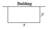
In this problem we want to maximize the area of a field and we know that will use 500 ft of fencing material. So, the area will be the function we are trying to optimize and the amount of fencing is the constraint. The two equations for these are,
\[\begin{align*}{\mbox{Maximize : }} & A = xy\\ {\mbox{Constraint : }} & 500 = x + 2y\end{align*}\]Okay, we know how to find the largest or smallest value of a function provided it’s only got a single variable. The area function (as well as the constraint) has two variables in it and so what we know about finding absolute extrema won’t work. However, if we solve the constraint for one of the two variables we can substitute this into the area and we will then have a function of a single variable.
So, let’s solve the constraint for \(x\). Note that we could have just as easily solved for \(y\) but that would have led to fractions and so, in this case, solving for \(x\) will probably be best.
\[x = 500 - 2y\]Substituting this into the area function gives a function of \(y\).
\[A\left( y \right) = \left( {500 - 2y} \right)y = 500y - 2{y^2}\]Now we want to find the largest value this will have on the interval \(\left[ {0,250} \right]\). The limits in this interval corresponds to taking \(y = 0\) (i.e. no sides to the fence) and \(y = 250\) (i.e. only two sides and no width, also if there are two sides each must be 250 ft to use the whole 500ft).
Note that the endpoints of the interval won’t make any sense from a physical standpoint if we actually want to enclose some area because they would both give zero area. They do, however, give us a set of limits on \(y\) and so the Extreme Value Theorem tells us that we will have a maximum value of the area somewhere between the two endpoints. Having these limits will also mean that we can use the process we discussed in the Finding Absolute Extrema section earlier in the chapter to find the maximum value of the area.
So, recall that the maximum value of a continuous function (which we’ve got here) on a closed interval (which we also have here) will occur at critical points and/or end points. As we’ve already pointed out the end points in this case will give zero area and so don’t make any sense. That means our only option will be the critical points.
So, let’s get the derivative and find the critical points.
\[A'\left( y \right) = 500 - 4y\]Setting this equal to zero and solving gives a lone critical point of \(y = 125\). Plugging this into the area gives an area of \(A\left( {125} \right) = 31250\,{\mbox{f}}{{\mbox{t}}^2}\). So according to the method from Absolute Extrema section this must be the largest possible area, since the area at either endpoint is zero.
Finally, let’s not forget to get the value of \(x\) and then we’ll have the dimensions since this is what the problem statement asked for. We can get the \(x\) by plugging in our \(y\) into the constraint.
\[x = 500 - 2\left( {125} \right) = 250\]The dimensions of the field that will give the largest area, subject to the fact that we used exactly 500 ft of fencing material, are 250 x 125.
Don’t forget to actually read the problem and give the answer that was asked for. These types of problems can take a fair amount of time/effort to solve and it’s not hard to sometimes forget what the problem was actually asking for.
In the previous problem we used the method from the Finding Absolute Extrema section to find the maximum value of the function we wanted to optimize. However, as we’ll see in later examples it will not always be easy to find endpoints. Also, even if we can find the endpoints we will see that sometimes dealing with the endpoints may not be easy either. Not only that, but this method requires that the function we’re optimizing be continuous on the interval we’re looking at, including the endpoints, and that may not always be the case.
So, before proceeding with any more examples let’s spend a little time discussing some methods for determining if our solution is in fact the absolute minimum/maximum value that we’re looking for. In some examples all of these will work while in others one or more won’t be all that useful. However, we will always need to use some method for making sure that our answer is in fact that optimal value that we’re after.
Method 1 : Use the method used in Finding Absolute Extrema.
This is the method used in the first example above. Recall that in order to use this method the interval of possible values of the independent variable in the function we are optimizing, let’s call it \(I\), must have finite endpoints. Also, the function we’re optimizing (once it’s down to a single variable) must be continuous on \(I\), including the endpoints. If these conditions are met then we know that the optimal value, either the maximum or minimum depending on the problem, will occur at either the endpoints of the range or at a critical point that is inside the range of possible solutions.
There are two main issues that will often prevent this method from being used however. First, not every problem will actually have a range of possible solutions that have finite endpoints at both ends. We’ll see at least one example of this as we work through the remaining examples. Also, many of the functions we’ll be optimizing will not be continuous once we reduce them down to a single variable and this will prevent us from using this method.
Method 2 : Use a variant of the First Derivative Test.
In this method we also will need an interval of possible values of the independent variable in the function we are optimizing, \(I\). However, in this case, unlike the previous method the endpoints do not need to be finite. Also, we will need to require that the function be continuous on the interior of the interval \(I\) and we will only need the function to be continuous at the end points if the endpoint is finite and the function actually exists at the endpoint. We’ll see several problems where the function we’re optimizing doesn’t actually exist at one of the endpoints. This will not prevent this method from being used.
Let’s suppose that \(x = c\) is a critical point of the function we’re trying to optimize, \(f\left( x \right)\). We already know from the First Derivative Test that if \(f'\left( x \right) > 0\) immediately to the left of \(x = c\) (i.e. the function is increasing immediately to the left) and if \(f'\left( x \right) < 0\) immediately to the right of \(x = c\)(i.e. the function is decreasing immediately to the right) then \(x = c\) will be a relative maximum for \(f\left( x \right)\).
Now, this does not mean that the absolute maximum of \(f\left( x \right)\) will occur at \(x = c\). However, suppose that we knew a little bit more information. Suppose that in fact we knew that \(f'\left( x \right) > 0\) for all \(x\) in \(I\) such that \(x < c\). Likewise, suppose that we knew that \(f'\left( x \right) < 0\) for all \(x\) in \(I\) such that \(x > c\). In this case we know that to the left of \(x = c\), provided we stay in \(I\) of course, the function is always increasing and to the right of \(x = c\), again staying in \(I\), we are always decreasing. In this case we can say that the absolute maximum of \(f\left( x \right)\) in \(I\) will occur at \(x = c\).
Similarly, if we know that to the left of \(x = c\) the function is always decreasing and to the right of \(x = c\) the function is always increasing then the absolute minimum of \(f\left( x \right)\) in \(I\) will occur at \(x = c\).
Before we give a summary of this method let’s discuss the continuity requirement a little. Nowhere in the above discussion did the continuity requirement apparently come into play. We require that the function we’re optimizing to be continuous in \(I\) to prevent the following situation.
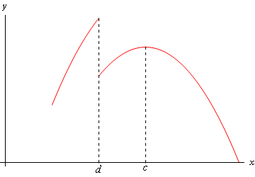
In this case, a relative maximum of the function clearly occurs at \(x = c\). Also, the function is always decreasing to the right and is always increasing to the left. However, because of the discontinuity at \(x = d\), we can clearly see that \(f\left( d \right) > f\left( c \right)\) and so the absolute maximum of the function does not occur at \(x = c\). Had the discontinuity at \(x = d\) not been there this would not have happened and the absolute maximum would have occurred at \(x = c\).
Here is a summary of this method.
First Derivative Test for Absolute Extrema
Let \(I\) be the interval of all possible values of \(x\) in \(f\left( x \right)\), the function we want to optimize, and further suppose that \(f\left( x \right)\) is continuous on \(I\) , except possibly at the endpoints. Finally suppose that \(x = c\) is a critical point of \(f\left( x \right)\) and that \(c\) is in the interval \(I\). If we restrict \(x\) to values from \(I\) (i.e. we only consider possible optimal values of the function) then,
- If \(f'\left( x \right) > 0\) for all \(x < c\) and if \(f'\left( x \right) < 0\) for all \(x > c\) then \(f\left( c \right)\) will be the absolute maximum value of \(f\left( x \right)\) on the interval \(I\).
- If \(f'\left( x \right) < 0\) for all \(x < c\) and if \(f'\left( x \right) > 0\) for all \(x > c\) then \(f\left( c \right)\) will be the absolute minimum value of \(f\left( x \right)\) on the interval \(I\).
Method 3 : Use the second derivative.
There are actually two ways to use the second derivative to help us identify the optimal value of a function and both use the Second Derivative Test to one extent or another.
The first way to use the second derivative doesn’t actually help us to identify the optimal value. What it does do is allow us to potentially exclude values and knowing this can simplify our work somewhat and so is not a bad thing to do.
Suppose that we are looking for the absolute maximum of a function and after finding the critical points we find that we have multiple critical points. Let’s also suppose that we run all of them through the second derivative test and determine that some of them are in fact relative minimums of the function. Since we are after the absolute maximum we know that a maximum (of any kind) can’t occur at relative minimums and so we immediately know that we can exclude these points from further consideration. We could do a similar check if we were looking for the absolute minimum. Doing this may not seem like all that great of a thing to do, but it can, on occasion, lead to a nice reduction in the amount of work that we need to do in later steps.
The second way of using the second derivative to identify the optimal value of a function is in fact very similar to the second method above. In fact, we will have the same requirements for this method as we did in that method. We need an interval of possible values of the independent variable in function we are optimizing, call it \(I\) as before, and the endpoint(s) may or may not be finite. We’ll also need to require that the function, \(f\left( x \right)\) be continuous everywhere in \(I\) except possibly at the endpoints as above.
Now, suppose that \(x = c\) is a critical point and that \(f''\left( c \right) > 0\). The second derivative test tells us that \(x = c\) must be a relative minimum of the function. Suppose however that we also knew that \(f''\left( x \right) > 0\) for all \(x\) in \(I\). In this case we would know that the function was concave up in all of \(I\) and that would in turn mean that the absolute minimum of \(f\left( x \right)\) in \(I\) would in fact have to be at \(x = c\).
Likewise, if \(x = c\) is a critical point and \(f''\left( x \right) < 0\) for all \(x\) in \(I\) then we would know that the function was concave down in \(I\) and that the absolute maximum of \(f\left( x \right)\) in \(I\) would have to be at \(x = c\).
Here is a summary of this method.
Second Derivative Test for Absolute Extrema
Let \(I\) be the interval of all possible values of \(x\) in \(f\left( x \right)\), the function we want to optimize, and suppose that \(f\left( x \right)\) is continuous on \(I\) , except possibly at the endpoints. Finally suppose that \(x = c\) is a critical point of \(f\left( x \right)\) and that \(c\) is in the interval \(I\). Then,
- If \(f''\left( x \right) > 0\) for all \(x\) in \(I\) then \(f\left( c \right)\) will be the absolute minimum value of \(f\left( x \right)\) on the interval \(I\).
- If \(f''\left( x \right) < 0\) for all \(x\) in \(I\) then \(f\left( c \right)\) will be the absolute maximum value of \(f\left( x \right)\) on the interval \(I\).
As we work examples over the next two sections we will use each of these methods as needed in the examples. In some cases, the method we use will be the only method we could use, in others it will be the easiest method to use and in others it will simply be the method we chose to use for that example. It is important to realize that we won’t be able to use each of the methods for every example. With some examples one method will be easiest to use or may be the only method that can be used, however, each of the methods described above will be used at least a couple of times through out all of the examples.
It is also important to be aware that some problems don’t allow any of the methods discussed above to be used exactly as outlined above. We may need to modify one of them or use a combination of them to fully work the problem. There is an example in the next section where none of the methods above work easily, although we do also present an alternative solution method in which we can use at least one of the methods discussed above.
Next, the vast majority of the examples worked over the course of the next section will only have a single critical point. Problems with more than one critical point are often difficult to know which critical point(s) give the optimal value. There are a couple of examples in the next two sections with more than one critical point including one in the next section mentioned above in which none of the methods discussed above easily work. In that example you can see some of the ideas you might need to do in order to find the optimal value.
Finally, in all of the methods above we referenced an interval \(I\). This was done to make the discussion a little easier. However, in all of the examples over the next two sections we will never explicitly say “this is the interval \(I\)”. Just remember that the interval \(I\) is just the largest interval of possible values of the independent variable in the function we are optimizing.
Okay, let’s work some more examples.
First, a quick figure (probably not to scale…).
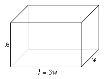
We want to minimize the cost of the materials subject to the constraint that the volume must be 50ft3. Note as well that the cost for each side is just the area of that side times the appropriate cost.
The two functions we’ll be working with here this time are,
\[\begin{align*}{\mbox{Minimize : }} & C = 10\left( {2lw} \right) + 6\left( {2wh + 2lh} \right)\, = 60{w^2} + 48wh\\ {\mbox{Constraint :}}& 50 = lwh = 3{w^2}h\end{align*}\]As with the first example, we will solve the constraint for one of the variables and plug this into the cost. It will definitely be easier to solve the constraint for \(h\) so let’s do that.
\[h = \frac{{50}}{{3{w^2}}}\]Plugging this into the cost gives,
\[C\left( w \right) = 60{w^2} + 48w\left( {\frac{{50}}{{3{w^2}}}} \right) = 60{w^2} + \frac{{800}}{w}\]Now, let’s get the first and second (we’ll be needing this later…) derivatives,
\[C'\left( w \right) = 120w - 800{w^{ - 2}} = \frac{{120{w^3} - 800}}{{{w^2}}}\hspace{0.25in}\hspace{0.25in}C''\left( w \right) = 120 + 1600{w^{ - 3}}\]Now we need the critical point(s) for the cost function. First, notice that \(w = 0\) is not a critical point. Clearly the derivative does not exist at \(w = 0\) but then neither does the function and remember that values of \(w\) will only be critical points if the function also exists at that point. Note that there is also a physical reason to avoid \(w = 0\). We are constructing a box and it would make no sense to have a zero width of the box.
So it looks like the only critical point will come from determining where the numerator is zero.
\[120{w^3} - 800 = 0\hspace{0.25in} \Rightarrow \hspace{0.25in}\,\,w = \sqrt[3]{{\frac{{800}}{{120}}}} = \sqrt[3]{{\frac{{20}}{3}}} = 1.8821\]So, we’ve got a single critical point and we now have to verify that this is in fact the value that will give the absolute minimum cost.
In this case we can’t use Method 1 from above. First, the function is not continuous at one of the endpoints, \(w = 0\), of our interval of possible values, i.e. \(w > 0\). Secondly, there is no theoretical upper limit to the width that will give a box with volume of 50 ft3. If \(w\) is very large then we would just need to make \(h\) very small.
The second method listed above would work here, but that’s going to involve some calculations, not difficult calculations, but more work nonetheless.
The third method however, will work quickly and simply here. First, we know that whatever the value of \(w\) that we get it will have to be positive and we can see second derivative above that provided \(w > 0\) we will have \(C''\left( w \right) > 0\) and so in the interval of possible optimal values the cost function will always be concave up and so \(w = 1.8821\) must give the absolute minimum cost.
All we need to do now is to find the remaining dimensions.
\[\begin{align*}w & = 1.8821\\ l & = 3w = 3\left( {1.8821} \right) = 5.6463\\ h & = \frac{{50}}{{3{w^2}}} = \frac{{50}}{{3{{\left( {1.8821} \right)}^2}}} = 4.7050\end{align*}\]Also, even though it was not asked for, the minimum cost is : \(C\left( {1.8821} \right) = \$ 637.60\).
This example is in many ways the exact opposite of the previous example. In this case we want to optimize the volume and the constraint this time is the amount of material used. We don’t have a cost here, but if you think about it the cost is nothing more than the amount of material used times a cost and so the amount of material and cost are pretty much tied together. If you can do one you can do the other as well. Note as well that the amount of material used is really just the surface area of the box.
As always, let’s start off with a quick sketch of the box.
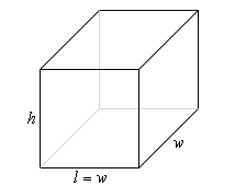
Now, as mentioned above we want to maximize the volume and the amount of material is the constraint so here are the equations we’ll need.
\[\begin{align*}{\mbox{Maximize : }} & V = lwh = {w^2}h\\ {\mbox{Constraint :}} & 10 = 2lw + 2wh + 2lh\, = 2{w^2} + 4wh\end{align*}\]We’ll solve the constraint for \(h\) and plug this into the equation for the volume.
\[h = \frac{{10 - 2{w^2}}}{{4w}} = \frac{{5 - {w^2}}}{{2w}}\hspace{0.25in}\hspace{0.25in} \Rightarrow \hspace{0.25in}\,\,\,\,\,\,\,V\left( w \right) = {w^2}\left( {\frac{{5 - {w^2}}}{{2w}}} \right) = \frac{1}{2}\left( {5w - {w^3}} \right)\]Here are the first and second derivatives of the volume function.
\[V'\left( w \right) = {{1 \over 2}}\left( {5 - 3{w^2}} \right)\hspace{0.25in}\hspace{0.25in}\hspace{0.25in}V''\left( w \right) = - 3w\]Note as well here that provided \(w > 0\), which from a physical standpoint we know must be true for the width of the box, then the volume function will be concave down and so if we get a single critical point then we know that it will have to be the value that gives the absolute maximum.
Setting the first derivative equal to zero and solving gives us the two critical points,
\[w = \pm \,\sqrt {\frac{5}{3}} = \pm \,1.2910\]In this case we can exclude the negative critical point since we are dealing with a length of a box and we know that these must be positive. Do not however get into the habit of just excluding any negative critical point. There are problems where negative critical points are perfectly valid possible solutions.
Now, as noted above we got a single critical point, 1.2910, and so this must be the value that gives the maximum volume and since the maximum volume is all that was asked for in the problem statement the answer is then : \[V\left( {1.2910} \right) = 2.1517\,{{\mbox{m}}^3}\].
Note that we could also have noted here that if \(0 < w < 1.2910\) then \(V'\left( w \right) > 0\) (using a test point we have \(V'\left( 1 \right) = 1 > 0\)) and likewise if \(w > 1.2910\) then \(V'\left( w \right) < 0\) (using a test point we have \(V'\left( 2 \right) = - {\frac{7}{2}} < 0\)) and so if we are to the left of the critical point the volume is always increasing and if we are to the right of the critical point the volume is always decreasing and so by the Method 2 above we can also see that the single critical point must give the absolute maximum of the volume.
Finally, even though these weren’t asked for here are the dimension of the box that gives the maximum volume.
\[l = w = 1.2910\hspace{1.0in}h = \frac{{5 - {{1.2910}^2}}}{{2\left( {1.2910} \right)}} = 1.2910\]So, it looks like in this case we actually have a perfect cube.
In the last two examples we’ve seen that many of these optimization problems can be done in both directions so to speak. In both examples we have essentially the same two equations: volume and surface area. However, in Example 2 the volume was the constraint and the cost (which is directly related to the surface area) was the function we were trying to optimize. In Example 3, on the other hand, we were trying to optimize the volume and the surface area was the constraint.
It is important to not get so locked into one way of doing these problems that we can’t do it in the opposite direction as needed as well. This is one of the more common mistakes that students make with these kinds of problems. They see one problem and then try to make every other problem that seems to be the same conform to that one solution even if the problem needs to be worked differently. Keep an open mind with these problems and make sure that you understand what is being optimized and what the constraint is before you jump into the solution.
Also, as seen in the last example we used two different methods of verifying that we did get the optimal value. Do not get too locked into one method of doing this verification that you forget about the other methods.
Let’s work some another example that this time doesn’t involve a rectangle or box.
Before starting the solution let’s first address the fact that we are using liters for volume. Because we want length measurements for the radius and height we’ll also need the volume to in terms of a length measurement. We can easily do this using the fact that 1 Liter = 1000 cm3 and so we can convert 1.5 liters into 1500 cm3. This will in turn give a radius and height in terms of centimeters.
In this problem the constraint is the volume and we want to minimize the amount of material used. This means that what we want to minimize is the surface area of the can and we’ll need to include both the walls of the can as well as the top and bottom “caps”. Here is a quick sketch to get us started off.
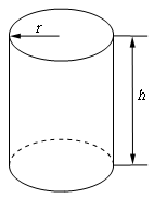
We’ll need the surface area of this can and that will be the surface area of the walls of the can (which is really just a cylinder) and the area of the top and bottom caps (which are just disks, and don’t forget that there are two of them).
Note that if you think of a cylinder of height \(h\) and radius \(r\) as just a bunch of disks/circles of radius \(r\) stacked on top of each other the equations for the surface area and volume are pretty simple to remember. The volume is just the area of each of the disks times the height. Similarly, the surface area of the walls of the cylinder is just the circumference of each circle times the height. We also can’t forget to add in the area of the two caps, \(\pi {r^2}\), to the total surface area.
So, the equation for the volume and surface area of the walls of a cylinder are then,
\[V = \left( {\pi {r^2}} \right)\left( h \right) = \pi {r^2}h\hspace{0.25in}\hspace{0.25in}\hspace{0.25in}A = \left( {2\pi r} \right)\left( h \right) = 2\pi rh\]Adding the surface area of the caps of the cylinder to the surface area the equations that we’ll need for this problem are,
\[\begin{align*}{\mbox{Minimize : }} & A = 2\pi rh + 2\pi {r^2}\\ {\mbox{Constraint :}} & 1500 = \pi {r^2}h\end{align*}\]In this case it looks like our best option is to solve the constraint for \(h\) and plug this into the area function.
\[h = \frac{{1500}}{{\pi {r^2}}}\hspace{0.25in} \Rightarrow \hspace{0.25in}A\left( r \right) = 2\pi r\left( {\frac{{1500}}{{\pi {r^2}}}} \right) + 2\pi {r^2} = 2\pi {r^2} + \frac{{3000}}{r}\]Notice that this formula will only make sense from a physical standpoint if \(r > 0\) which is a good thing as it is not defined at \(r = 0\).
Next, let’s get the first derivative.
\[A'\left( r \right) = 4\pi r - \frac{{3000}}{{{r^2}}} = \frac{{4\pi {r^3} - 3000}}{{{r^2}}}\]From this we can see that we have one critical points : \(r = \sqrt[3]{\frac{750}{\pi}} = 6.2035\)(where the derivative is zero). Note that \(r = 0\) is not a critical point because the area function does not exist there, which makes sense from a physical standpoint as well given that we know that \(r\) must be positive in order to actually have a can.
So, we only have a single critical point to deal with here and notice that 6.2035 is the only value for which the derivative will be zero and hence the only place (with \(r > 0\) of course) that the derivative may change sign. It’s not difficult, using test points, to check that if \(0 < r < 6.2035\) then \(A'\left( r \right) < 0\) and likewise if \(r > 6.2035\) then \(A'\left( r \right) > 0\). The variant of the First Derivative Test above then tells us that the absolute minimum value of the area (for \(r > 0\)) must occur at \[r = 6.2035\].
All we need to do this is determine height of the can and we’ll be done.
\[h = \frac{{1500}}{{\pi {{\left( {6.2035} \right)}^2}}} = 12.4070\]Therefore, if the manufacturer makes the can with a radius of 6.2035 cm and a height of 12.4070 cm the least amount of material will be used to make the can.
As an interesting side problem and extension to the above example you might want to show that for a given volume, \(L\), the minimum material will be used if \(h = 2r\) regardless of the volume of the can.
In the examples to this point we’ve put in quite a bit of discussion in the solution. In the remaining problems we won’t be putting in quite as much discussion and leave it to you to fill in any missing details.
Let’s let the height of the box be \(h\). So, the width/length of the corners being cut out is also \(h\) and so the vertical side will have a “new” height of \(10 - 2h\) and the horizontal side will have a “new” width of \(14 - 2h\). Here is a sketch with all this information put in,
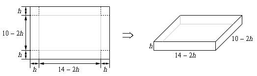
In this example, for the first time, we’ve run into a problem where the constraint doesn’t really have an equation. The constraint is simply the size of the piece of cardboard and has already been factored into the figure above. This will happen on occasion and so don’t get excited about it when it does. This just means that we have one less equation to worry about. In this case we want to maximize the volume. Here is the volume, in terms of \(h\) and its first derivative.
\[V\left( h \right) = h\left( {14 - 2h} \right)\left( {10 - 2h} \right) = 140h - 48{h^2} + 4{h^3}\hspace{0.25in}\hspace{0.25in}V'\left( h \right) = 140 - 96h + 12{h^2}\]Setting the first derivative equal to zero and solving gives the following two critical points,
\[h = \frac{{12 \pm \sqrt {39} }}{3} = 1.9183,\,\,\,\,6.0817\]We now have an apparent problem. We have two critical points and we’ll need to determine which one is the value we need. The fact that we have two critical points means that neither the first derivative test or the second derivative test can be used here as they both require a single critical point. This isn’t a real problem however. Go back to the figure at the start of the solution and notice that we can quite easily find limits on \(h\). The smallest \(h\) can be is \(h = 0\) even though this doesn’t make much sense as we won’t get a box in this case. Also, from the 10 inch side we can see that the largest \(h\) can be is \(h = 5\) although again, this doesn’t make much sense physically.
So, knowing that whatever \(h\) is it must be in the range \(0 \le h \le 5\) we can see that the second critical point is outside this range and so the only critical point that we need to worry about is 1.9183.
Finally, since the volume is defined and continuous on \(0 \le h \le 5\) all we need to do is plug in the critical points and endpoints into the volume to determine which gives the largest volume. Here are those function evaluations.
\[V\left( 0 \right) = 0\hspace{0.25in}\hspace{0.25in}V\left( {1.9183} \right) = 120.1644\hspace{0.25in}\hspace{0.25in}V\left( 5 \right) = 0\]So, if we take \(h = 1.9183\) we get a maximum volume.

This problem is a little different from the previous problems. Both the constraint and the function we are going to optimize are areas. The constraint is that the overall area of the poster must be 200 in2 while we want to optimize the printed area (i.e. the area of the poster with the margins taken out).
Let’s define the height of the poster to be \(h\) and the width of the poster to be \(w\). Here is a new sketch of the poster and we can see that once we’ve taken the margins into account the width of the printed area is \(w - 2\) and the height of the printer area is \(h - 3.5\).
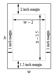
Here are the equations that we’ll be working with.
\[\begin{align*}{\mbox{Maximize : }} & A = \left( {w - 2} \right)\left( {h - 3.5} \right)\\ {\mbox{Constraint :}} & 200 = wh\end{align*}\]Solving the constraint for \(h\) and plugging into the equation for the printed area gives,
\[A\left( w \right) = \left( {w - 2} \right)\left( {\frac{{200}}{w} - 3.5} \right) = 207 - 3.5w - \frac{{400}}{w}\]The first and second derivatives are,
\[A'\left( w \right) = - 3.5 + \frac{{400}}{{{w^2}}} = \frac{{400 - 3.5{w^2}}}{{{w^2}}}\hspace{0.25in}\hspace{0.25in}A''\left( w \right) = - \frac{{800}}{{{w^3}}}\]From the first derivative we have the following two critical points (\(w = 0\) is not a critical point because the area function does not exist there).
\[w = \pm \,\sqrt {\frac{400}{3.5}} = \pm \,10.6904\]However, since we’re dealing with the dimensions of a piece of paper we know that we must have \(w > 0\) and so only 10.6904 will make sense.
Also notice that provided \(w > 0\) the second derivative will always be negative and so in the range of possible optimal values of the width the area function is always concave down and so we know that the maximum printed area will be at \(w = 10.6904\,\,{\mbox{inches}}\).
The height of the paper that gives the maximum printed area is then,
\[h = \frac{{200}}{{10.6904}} = 18.7084\,\,{\mbox{inches}}\]We’ve worked quite a few examples to this point and we have quite a few more to work. However, this section has gotten quite lengthy so let’s continue our examples in the next section. This is being done mostly because these notes are also being presented on the web and this will help to keep the load times on the pages down somewhat.