Section 2.8 : Equilibrium Solutions
In the previous section we modeled a population based on the assumption that the growth rate would be a constant. However, in reality this doesn’t make much sense. Clearly a population cannot be allowed to grow forever at the same rate. The growth rate of a population needs to depend on the population itself. Once a population reaches a certain point the growth rate will start reduce, often drastically. A much more realistic model of a population growth is given by the logistic growth equation. Here is the logistic growth equation.
\[P' = r\left( {1 - \frac{P}{K}} \right)P\]In the logistic growth equation \(r\) is the intrinsic growth rate and is the same \(r\) as in the last section. In other words, it is the growth rate that will occur in the absence of any limiting factors. \(K\) is called either the saturation level or the carrying capacity.
Now, we claimed that this was a more realistic model for a population. Let’s see if that in fact is correct. To allow us to sketch a direction field let’s pick a couple of numbers for \(r\) and \(K\). We’ll use \(r = \frac{1}{2}\) and \(K = 10\). For these values the logistics equation is.
\[P' = \frac{1}{2}\left( {1 - \frac{P}{{10}}} \right)P\]If you need a refresher on sketching direction fields go back and take a look at that section. First notice that the derivative will be zero at \(P = 0\) and \(P = 10\). Also notice that these are in fact solutions to the differential equation. These two values are called equilibrium solutions since they are constant solutions to the differential equation. We’ll leave the rest of the details on sketching the direction field to you. Here is the direction field as well as a couple of solutions sketched in as well.
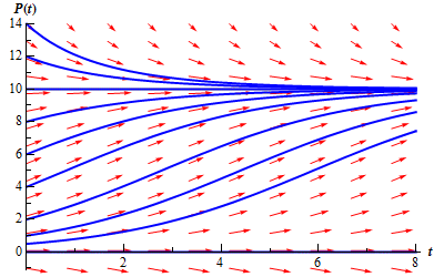
Note, that we included a small portion of negative \(P\)’s in here even though they really don’t make any sense for a population problem. The reason for this will be apparent down the road. Also, notice that a population of say 8 doesn’t make all that much sense so let’s assume that population is in thousands or millions so that 8 actually represents 8,000 or 8,000,000 individuals in a population.
Notice that if we start with a population of zero, there is no growth and the population stays at zero. So, the logistic equation will correctly figure out that. Next, notice that if we start with a population in the range \(0 < P\left( 0 \right) < 10\) then the population will grow, but start to level off once we get close to a population of 10. If we start with a population of 10, the population will stay at 10. Finally, if we start with a population that is greater than 10, then the population will actually die off until we start nearing a population of 10, at which point the population decline will start to slow down.
Now, from a realistic standpoint this should make some sense. Populations can’t just grow forever without bound. Eventually the population will reach such a size that the resources of an area are no longer able to sustain the population and the population growth will start to slow as it comes closer to this threshold. Also, if you start off with a population greater than what an area can sustain there will actually be a die off until we get near to this threshold.
In this case that threshold appears to be 10, which is also the value of \(K\) for our problem. That should explain the name that we gave \(K\) initially. The carrying capacity or saturation level of an area is the maximum sustainable population for that area.
So, the logistics equation, while still quite simplistic, does a much better job of modeling what will happen to a population.
Now, let’s move on to the point of this section. The logistics equation is an example of an autonomous differential equation. Autonomous differential equations are differential equations that are of the form.
\[\frac{{dy}}{{dt}} = f\left( y \right)\]The only place that the independent variable, \(t\) in this case, appears is in the derivative.
Notice that if \(f\left( {{y_0}} \right) = 0\) for some value \(y = {y_0}\) then this will also be a solution to the differential equation. These values are called equilibrium solutions or equilibrium points. What we would like to do is classify these solutions. By classify we mean the following. If solutions start “near” an equilibrium solution will they move away from the equilibrium solution or towards the equilibrium solution? Upon classifying the equilibrium solutions we can then know what all the other solutions to the differential equation will do in the long term simply by looking at which equilibrium solutions they start near.
So, just what do we mean by “near”? Go back to our logistics equation.
\[P' = \frac{1}{2}\left( {1 - \frac{P}{{10}}} \right)P\]As we pointed out there are two equilibrium solutions to this equation \(P = 0\) and \(P = 10\). If we ignore the fact that we’re dealing with population these points break up the \(P\) number line into three distinct regions.
\[ - \infty < P < 0\hspace{0.25in}\hspace{0.25in}\hspace{0.25in}\,\,\,\,0 < P < 10\hspace{0.25in}\hspace{0.25in}\hspace{0.25in}\,10 < P < \infty \]We will say that a solution starts “near” an equilibrium solution if it starts in a region that is on either side of that equilibrium solution. So, solutions that start “near” the equilibrium solution \(P = 10\) will start in either
\[0 < P < 10\hspace{0.25in}{\mbox{OR}}\hspace{0.25in}\,10 < P < \infty \]and solutions that start “near” \(P = 0\) will start in either
\[ - \infty < P < 0\hspace{0.25in}\,\,\,{\mbox{OR}}\hspace{0.25in}\,\,\,\,\,\,0 < P < 10\]For regions that lie between two equilibrium solutions we can think of any solutions starting in that region as starting “near” either of the two equilibrium solutions as we need to.
Now, solutions that start “near” \(P = 0\) all move away from the solution as \(t\) increases. Note that moving away does not necessarily mean that they grow without bound as they move away. It only means that they move away. Solutions that start out greater than \(P = 0\) move away but do stay bounded as \(t\) grows. In fact, they move in towards \(P = 10\).
Equilibrium solutions in which solutions that start “near” them move away from the equilibrium solution are called unstable equilibrium points or unstable equilibrium solutions. So, for our logistics equation, \(P = 0\) is an unstable equilibrium solution.
Next, solutions that start “near” \(P = 10\) all move in toward \(P = 10\) as \(t\) increases. Equilibrium solutions in which solutions that start “near” them move toward the equilibrium solution are called asymptotically stable equilibrium points or asymptotically stable equilibrium solutions. So, \(P = 10\) is an asymptotically stable equilibrium solution.
There is one more classification, but I’ll wait until we get an example in which this occurs to introduce it. So, let’s take a look at a couple of examples.
First, find the equilibrium solutions. This is generally easy enough to do.
\[{y^2} - y - 6 = \left( {y - 3} \right)\left( {y + 2} \right) = 0\]So, it looks like we’ve got two equilibrium solutions. Both \(y = -2\) and \(y = 3\) are equilibrium solutions. Below is the sketch of some integral curves for this differential equation. A sketch of the integral curves or direction fields can simplify the process of classifying the equilibrium solutions.
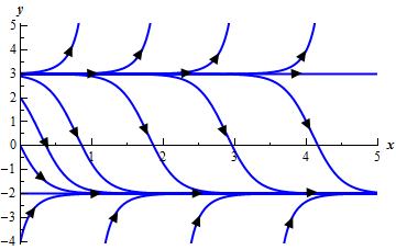
From this sketch it appears that solutions that start “near” \(y = -2\) all move towards it as \(t\) increases and so \(y = -2\) is an asymptotically stable equilibrium solution and solutions that start “near” \(y = 3\) all move away from it as \(t\) increases and so \(y = 3\) is an unstable equilibrium solution.
This next example will introduce the third classification that we can give to equilibrium solutions.
The equilibrium solutions to this differential equation are \(y = -2\), \(y = 2\), and \(y = -1\). Below is the sketch of the integral curves.
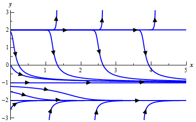
From this it is clear (hopefully) that \(y = 2\) is an unstable equilibrium solution and \(y = -2\) is an asymptotically stable equilibrium solution. However, \(y = -1\) behaves differently from either of these two. Solutions that start above it move towards \(y = -1\) while solutions that start below \(y = -1\) move away as \(t\) increases.
In cases where solutions on one side of an equilibrium solution move towards the equilibrium solution and on the other side of the equilibrium solution move away from it we call the equilibrium solution semi-stable.
So, \(y = -1\) is a semi-stable equilibrium solution.