Section 5.7 : Real Eigenvalues
It’s now time to start solving systems of differential equations. We’ve seen that solutions to the system,
\[\vec x' = A\vec x\]will be of the form
\[\vec x = \vec \eta {{\bf{e}}^{\lambda t}}\]where \(\lambda\) and \(\vec \eta \)are eigenvalues and eigenvectors of the matrix \(A\). We will be working with \(2 \times 2\) systems so this means that we are going to be looking for two solutions, \({\vec x_1}\left( t \right)\) and \({\vec x_2}\left( t \right)\), where the determinant of the matrix,
\[X = \left( {{{\vec x}_1}\,\,\,{{\vec x}_2}} \right)\]is nonzero.
We are going to start by looking at the case where our two eigenvalues, \({\lambda _{\,1}}\) and \({\lambda _{\,2}}\) are real and distinct. In other words, they will be real, simple eigenvalues. Recall as well that the eigenvectors for simple eigenvalues are linearly independent. This means that the solutions we get from these will also be linearly independent. If the solutions are linearly independent the matrix \(X\) must be nonsingular and hence these two solutions will be a fundamental set of solutions. The general solution in this case will then be,
\[\vec x\left( t \right) = {c_1}{{\bf{e}}^{{\lambda _1}t}}{\vec \eta ^{\left( 1 \right)}} + {c_2}{{\bf{e}}^{{\lambda _2}t}}{\vec \eta ^{\left( 2 \right)}}\]Note that each of our examples will actually be broken into two examples. The first example will be solving the system and the second example will be sketching the phase portrait for the system. Phase portraits are not always taught in a differential equations course and so we’ll strip those out of the solution process so that if you haven’t covered them in your class you can ignore the phase portrait example for the system.
So, the first thing that we need to do is find the eigenvalues for the matrix.
\[\begin{align*}\det \left( {A - \lambda I} \right) & = \left| {\begin{array}{*{20}{c}}{1 - \lambda }&2\\3&{2 - \lambda }\end{array}} \right|\\ & = {\lambda ^2} - 3\lambda - 4\\ & = \left( {\lambda + 1} \right)\left( {\lambda - 4} \right)\hspace{0.25in} \Rightarrow \hspace{0.25in}{\lambda _1} = - 1,\,\,{\lambda _2} = 4\end{align*}\]Now let’s find the eigenvectors for each of these.
\({\lambda _{\,1}} = - 1\) :
We’ll need to solve,
The eigenvector in this case is,
\[\vec \eta = \left( {\begin{array}{*{20}{c}}{ - {\eta _2}}\\{{\eta _2}}\end{array}} \right)\hspace{0.25in} \Rightarrow \hspace{0.25in}{\vec \eta ^{\left( 1 \right)}} = \left( {\begin{array}{*{20}{c}}{ - 1}\\1\end{array}} \right),\,\,\,\,\,\,\,{\eta _2} = 1\]\({\lambda _{\,2}} = 4\) :
We’ll need to solve,
The eigenvector in this case is,
\[\vec \eta = \left( {\begin{array}{*{20}{c}}{\frac{2}{3}{\eta _2}}\\{{\eta _2}}\end{array}} \right)\hspace{0.25in} \Rightarrow \hspace{0.25in}{\vec \eta ^{\left( 2 \right)}} = \left( {\begin{array}{*{20}{c}}2\\3\end{array}} \right),\,\,\,\,\,\,\,{\eta _2} = 3\]Then general solution is then,
\[\vec x\left( t \right) = {c_1}{{\bf{e}}^{ - t}}\left( {\begin{array}{*{20}{c}}{ - 1}\\1\end{array}} \right) + {c_2}{{\bf{e}}^{4t}}\left( {\begin{array}{*{20}{c}}2\\3\end{array}} \right)\]Now, we need to find the constants. To do this we simply need to apply the initial conditions.
\[\left( {\begin{array}{*{20}{c}}0\\{ - 4}\end{array}} \right) = \vec x\left( 0 \right) = {c_1}\left( {\begin{array}{*{20}{c}}{ - 1}\\1\end{array}} \right) + {c_2}\left( {\begin{array}{*{20}{c}}2\\3\end{array}} \right)\]All we need to do now is multiply the constants through and we then get two equations (one for each row) that we can solve for the constants. This gives,
\[\left. {\begin{array}{*{20}{c}}{ - {c_1} + 2{c_2} = 0}\\{{c_1} + 3{c_2} = - 4}\end{array}} \right\}\hspace{0.25in} \Rightarrow \hspace{0.25in}{c_1} = - \frac{8}{5},\,\,\,{c_2} = - \frac{4}{5}\]The solution is then,
\[\vec x\left( t \right) = - \frac{8}{5}{{\bf{e}}^{ - t}}\left( {\begin{array}{*{20}{c}}{ - 1}\\1\end{array}} \right) - \frac{4}{5}{{\bf{e}}^{4t}}\left( {\begin{array}{*{20}{c}}2\\3\end{array}} \right)\]Now, let’s take a look at the phase portrait for the system.
From the last example we know that the eigenvalues and eigenvectors for this system are,
\[\begin{align*}{\lambda _1} & = - 1 & \hspace{0.25in}{{\vec \eta }^{\left( 1 \right)}} & = \left( {\begin{array}{*{20}{c}}{ - 1}\\1\end{array}} \right)\\ {\lambda _2} & = 4 & \hspace{0.25in}{{\vec \eta }^{\left( 2 \right)}} & = \left( {\begin{array}{*{20}{c}}2\\3\end{array}} \right)\end{align*}\]It turns out that this is all the information that we will need to sketch the direction field. We will relate things back to our solution however so that we can see that things are going correctly.
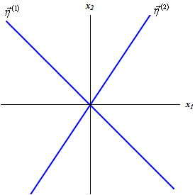
We’ll start by sketching lines that follow the direction of the two eigenvectors. This gives,
Now, from the first example our general solution is
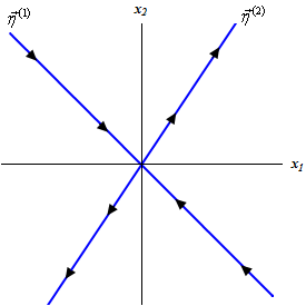
\[\vec x\left( t \right) = {c_1}{{\bf{e}}^{ - t}}\left( {\begin{array}{*{20}{c}}{ - 1}\\1\end{array}} \right) + {c_2}{{\bf{e}}^{4t}}\left( {\begin{array}{*{20}{c}}2\\3\end{array}} \right)\]If we have \({c_2} = 0\) then the solution is an exponential times a vector and all that the exponential does is affect the magnitude of the vector and the constant \(c_{1}\) will affect both the sign and the magnitude of the vector. In other words, the trajectory in this case will be a straight line that is parallel to the vector, \({\vec \eta ^{\left( 1 \right)}}\). Also notice that as \(t\) increases the exponential will get smaller and smaller and hence the trajectory will be moving in towards the origin. If \({c_1} > 0\) the trajectory will be in Quadrant II and if \({c_1} < 0\) the trajectory will be in Quadrant IV.
So, the line in the graph above marked with \({\vec \eta ^{\left( 1 \right)}}\) will be a sketch of the trajectory corresponding to \({c_2} = 0\) and this trajectory will approach the origin as \(t\) increases.
If we now turn things around and look at the solution corresponding to having \({c_1} = 0\) we will have a trajectory that is parallel to \({\vec \eta ^{\left( 2 \right)}}\). Also, since the exponential will increase as \(t\) increases and so in this case the trajectory will now move away from the origin as \(t\) increases. We will denote this with arrows on the lines in the graph above.
Notice that we could have gotten this information without actually going to the solution. All we really need to do is look at the eigenvalues. Eigenvalues that are negative will correspond to solutions that will move towards the origin as \(t\) increases in a direction that is parallel to its eigenvector. Likewise, eigenvalues that are positive move away from the origin as \(t\) increases in a direction that will be parallel to its eigenvector.
If both constants are in the solution we will have a combination of these behaviors. For large negative \(t\)’s the solution will be dominated by the portion that has the negative eigenvalue since in these cases the exponent will be large and positive. Trajectories for large negative \(t\)’s will be parallel to \({\vec \eta ^{\left( 1 \right)}}\) and moving in the same direction.
Solutions for large positive \(t\)’s will be dominated by the portion with the positive eigenvalue. Trajectories in this case will be parallel to \({\vec \eta ^{\left( 2 \right)}}\) and moving in the same direction.
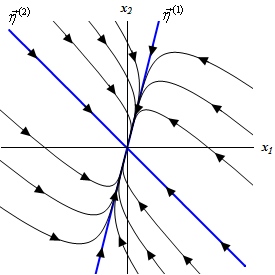
In general, it looks like trajectories will start “near” \({\vec \eta ^{\left( 1 \right)}}\), move in towards the origin and then as they get closer to the origin they will start moving towards \({\vec \eta ^{\left( 2 \right)}}\) and then continue up along this vector. Sketching some of these in will give the following phase portrait. Here is a sketch of this with the trajectories corresponding to the eigenvectors marked in blue.
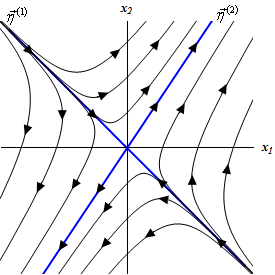
In this case the equilibrium solution \(\left( {0,0} \right)\) is called a saddle point and is unstable. In this case unstable means that solutions move away from it as \(t\) increases.
So, we’ve solved a system in matrix form, but remember that we started out without the systems in matrix form. Now let’s take a quick look at an example of a system that isn’t in matrix form initially.
We first need to convert this into matrix form. This is easy enough. Here is the matrix form of the system.
\[\vec x' = \left( {\begin{array}{*{20}{c}}1&2\\3&2\end{array}} \right)\vec x,\hspace{0.25in}\vec x\left( 0 \right) = \left( {\begin{array}{*{20}{c}}0\\{ - 4}\end{array}} \right)\]This is just the system from the first example and so we’ve already got the solution to this system. Here it is.
\[\vec x\left( t \right) = - \frac{8}{5}{{\bf{e}}^{ - t}}\left( {\begin{array}{*{20}{c}}{ - 1}\\1\end{array}} \right) - \frac{4}{5}{{\bf{e}}^{4t}}\left( {\begin{array}{*{20}{c}}2\\3\end{array}} \right)\]Now, since we want the solution to the system not in matrix form let’s go one step farther here. Let’s multiply the constants and exponentials into the vectors and then add up the two vectors.
\[\vec x\left( t \right) = \left( {\begin{array}{*{20}{c}}{\frac{8}{5}{{\bf{e}}^{ - t}}}\\{ - \frac{8}{5}{{\bf{e}}^{ - t}}}\end{array}} \right) - \left( {\begin{array}{*{20}{c}}{\frac{8}{5}{{\bf{e}}^{4t}}}\\{\frac{{12}}{5}{{\bf{e}}^{4t}}}\end{array}} \right) = \left( {\begin{array}{*{20}{c}}{\frac{8}{5}{{\bf{e}}^{ - t}} - \frac{8}{5}{{\bf{e}}^{4t}}}\\{ - \frac{8}{5}{{\bf{e}}^{ - t}} - \frac{{12}}{5}{{\bf{e}}^{4t}}}\end{array}} \right)\]Now, recall,
\[\vec x\left( t \right) = \left( {\begin{array}{*{20}{c}}{{x_1}\left( t \right)}\\{{x_2}\left( t \right)}\end{array}} \right)\]So, the solution to the system is then,
\[\begin{align*}{x_1}\left( t \right) & = \frac{8}{5}{{\bf{e}}^{ - t}} - \frac{8}{5}{{\bf{e}}^{4t}}\\ {x_2}\left( t \right) & = - \frac{8}{5}{{\bf{e}}^{ - t}} - \frac{{12}}{5}{{\bf{e}}^{4t}}\end{align*}\]Let’s work another example.
So, the first thing that we need to do is find the eigenvalues for the matrix.
\[\begin{align*}\det \left( {A - \lambda I} \right) & = \left| {\begin{array}{*{20}{c}}{ - 5 - \lambda }&1\\4&{ - 2 - \lambda }\end{array}} \right|\\ & = {\lambda ^2} + 7\lambda + 6\\ & = \left( {\lambda + 1} \right)\left( {\lambda + 6} \right)\hspace{0.25in} \Rightarrow \hspace{0.25in}{\lambda _1} = - 1,\,\,{\lambda _2} = - 6\end{align*}\]Now let’s find the eigenvectors for each of these.
\({\lambda _{\,1}} = - 1\) :
We’ll need to solve,
The eigenvector in this case is,
\[\vec \eta = \left( {\begin{array}{*{20}{c}}{{\eta _1}}\\{4{\eta _1}}\end{array}} \right)\hspace{0.25in} \Rightarrow \hspace{0.25in}{\vec \eta ^{\left( 1 \right)}} = \left( {\begin{array}{*{20}{c}}1\\4\end{array}} \right),\,\,\,\,\,\,\,{\eta _1} = 1\]\({\lambda _{\,2}} = - 6\) :
We’ll need to solve,
The eigenvector in this case is,
\[\vec \eta = \left( {\begin{array}{*{20}{c}}{ - {\eta _2}}\\{{\eta _2}}\end{array}} \right)\hspace{0.25in} \Rightarrow \hspace{0.25in}{\vec \eta ^{\left( 2 \right)}} = \left( {\begin{array}{*{20}{c}}{ - 1}\\1\end{array}} \right),\,\,\,\,\,\,\,{\eta _2} = 1\]Then general solution is then,
\[\vec x\left( t \right) = {c_1}{{\bf{e}}^{ - t}}\left( {\begin{array}{*{20}{c}}1\\4\end{array}} \right) + {c_2}{{\bf{e}}^{ - 6t}}\left( {\begin{array}{*{20}{c}}{ - 1}\\1\end{array}} \right)\]Now, we need to find the constants. To do this we simply need to apply the initial conditions.
\[\left( {\begin{array}{*{20}{c}}1\\2\end{array}} \right) = \vec x\left( 0 \right) = {c_1}\left( {\begin{array}{*{20}{c}}1\\4\end{array}} \right) + {c_2}\left( {\begin{array}{*{20}{c}}{ - 1}\\1\end{array}} \right)\]Now solve the system for the constants.
\[\left. {\begin{array}{*{20}{c}}{{c_1} - {c_2} = 1}\\{4{c_1} + {c_2} = 2}\end{array}} \right\}\hspace{0.25in} \Rightarrow \hspace{0.25in}{c_1} = \frac{3}{5},\,\,\,{c_2} = - \frac{2}{5}\]The solution is then,
\[\vec x\left( t \right) = \frac{3}{5}{{\bf{e}}^{ - t}}\left( {\begin{array}{*{20}{c}}1\\4\end{array}} \right) - \frac{2}{5}{{\bf{e}}^{ - 6t}}\left( {\begin{array}{*{20}{c}}{ - 1}\\1\end{array}} \right)\]Now let’s find the phase portrait for this system.
From the last example we know that the eigenvalues and eigenvectors for this system are,
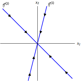
\[\begin{align*}{\lambda _1} & = - 1 & \hspace{0.25in}{{\vec \eta }^{\left( 1 \right)}} & = \left( {\begin{array}{*{20}{c}}1\\4\end{array}} \right)\\ {\lambda _2} & = - 6 & \hspace{0.25in}{{\vec \eta }^{\left( 2 \right)}} & = \left( {\begin{array}{*{20}{c}}{ - 1}\\1\end{array}} \right)\end{align*}\]This one is a little different from the first one. However, it starts in the same way. We’ll first sketch the trajectories corresponding to the eigenvectors. Notice as well that both of the eigenvalues are negative and so trajectories for these will move in towards the origin as \(t\) increases. When we sketch the trajectories we’ll add in arrows to denote the direction they take as \(t\) increases. Here is the sketch of these trajectories.
Now, here is where the slight difference from the first phase portrait comes up. All of the trajectories will move in towards the origin as \(t\) increases since both of the eigenvalues are negative. The issue that we need to decide upon is just how they do this. This is actually easier than it might appear to be at first.
The second eigenvalue is larger than the first. For large and positive \(t\)’s this means that the solution for this eigenvalue will be smaller than the solution for the first eigenvalue. Therefore, as \(t\) increases the trajectory will move in towards the origin and do so parallel to \({\vec \eta ^{\left( 1 \right)}}\). Likewise, since the second eigenvalue is larger than the first this solution will dominate for large and negative \(t\)’s. Therefore, as we decrease \(t\) the trajectory will move away from the origin and do so parallel to \({\vec \eta ^{\left( 2 \right)}}\).
Adding in some trajectories gives the following sketch.
In these cases we call the equilibrium solution \(\left( {0,0} \right)\) a node and it is asymptotically stable. Equilibrium solutions are asymptotically stable if all the trajectories move in towards it as \(t\) increases.
Note that nodes can also be unstable. In the last example if both of the eigenvalues had been positive all the trajectories would have moved away from the origin and in this case the equilibrium solution would have been unstable.
Before moving on to the next section we need to do one more example. When we first started talking about systems it was mentioned that we can convert a higher order differential equation into a system. We need to do an example like this so we can see how to solve higher order differential equations using systems.
So, we first need to convert this into a system. Here’s the change of variables,
\[\begin{align*}{x_1} & = y & \hspace{0.25in}{{x'}_1} & = y' = {x_2}\\ {x_2} & = y' & \hspace{0.25in}{{x'}_2} & = y'' = \frac{3}{2}y - \frac{5}{2}y' = \frac{3}{2}{x_1} - \frac{5}{2}{x_2}\end{align*}\]The system is then,
\[\vec x' = \left( {\begin{array}{*{20}{c}}0&1\\{\frac{3}{2}}&{ - \frac{5}{2}}\end{array}} \right)\vec x\hspace{0.25in}\vec x\left( 0 \right) = \left( {\begin{array}{*{20}{c}}{ - 4}\\9\end{array}} \right)\]where,
\[\vec x\left( t \right) = \left( {\begin{array}{*{20}{c}}{{x_1}\left( t \right)}\\{{x_2}\left( t \right)}\end{array}} \right) = \left( {\begin{array}{*{20}{c}}{y\left( t \right)}\\{y'\left( t \right)}\end{array}} \right)\]Now we need to find the eigenvalues for the matrix.
\[\begin{align*}\det \left( {A - \lambda I} \right) & = \left| {\begin{array}{*{20}{c}}{ - \lambda }&1\\{\frac{3}{2}}&{ - \frac{5}{2} - \lambda }\end{array}} \right|\\ & = {\lambda ^2} + \frac{5}{2}\lambda - \frac{3}{2}\\ & = \frac{1}{2}\left( {\lambda + 3} \right)\left( {2\lambda - 1} \right)\hspace{0.25in}{\lambda _1} = - 3,\,\,\,{\lambda _2} = \frac{1}{2}\end{align*}\]Now let’s find the eigenvectors.
\({\lambda _{\,1}} = - 3\) :
We’ll need to solve,
The eigenvector in this case is,
\[\vec \eta = \left( {\begin{array}{*{20}{c}}{{\eta _1}}\\{ - 3{\eta _1}}\end{array}} \right)\hspace{0.25in} \Rightarrow \hspace{0.25in}{\vec \eta ^{\left( 1 \right)}} = \left( {\begin{array}{*{20}{c}}1\\{ - 3}\end{array}} \right),\,\,\,\,\,\,\,{\eta _1} = 1\]\({\lambda _{\,2}} = \frac{1}{2}\):
We’ll need to solve,
The eigenvector in this case is,
\[\vec \eta = \left( {\begin{array}{*{20}{c}}{{\eta _1}}\\{\frac{1}{2}{\eta _1}}\end{array}} \right)\hspace{0.25in} \Rightarrow \hspace{0.25in}{\vec \eta ^{\left( 2 \right)}} = \left( {\begin{array}{*{20}{c}}2\\1\end{array}} \right),\,\,\,\,\,\,\,{\eta _1} = 2\]The general solution is then,
\[\vec x\left( t \right) = {c_1}{{\bf{e}}^{ - 3t}}\left( {\begin{array}{*{20}{c}}1\\{ - 3}\end{array}} \right) + {c_2}{{\bf{e}}^{\frac{t}{2}}}\left( {\begin{array}{*{20}{c}}2\\1\end{array}} \right)\]Apply the initial condition.
\[\left( {\begin{array}{*{20}{c}}{ - 4}\\9\end{array}} \right) = \vec x\left( 0 \right) = {c_1}\left( {\begin{array}{*{20}{c}}1\\{ - 3}\end{array}} \right) + {c_2}\left( {\begin{array}{*{20}{c}}2\\1\end{array}} \right)\]This gives the system of equations that we can solve for the constants.
\[\left. {\begin{array}{*{20}{c}}{{c_1} + 2{c_2} = - 4}\\{ - 3{c_1} + {c_2} = 9}\end{array}} \right\}\hspace{0.25in} \Rightarrow \hspace{0.25in}{c_1} = - \frac{{22}}{7},\,\,\,{c_2} = - \frac{3}{7}\]The actual solution to the system is then,
\[\vec x\left( t \right) = - \frac{{22}}{7}{{\bf{e}}^{ - 3t}}\left( {\begin{array}{*{20}{c}}1\\{ - 3}\end{array}} \right) - \frac{3}{7}{{\bf{e}}^{\frac{t}{2}}}\left( {\begin{array}{*{20}{c}}2\\1\end{array}} \right)\]Now recalling that,
\[\vec x\left( t \right) = \left( {\begin{array}{*{20}{c}}{y\left( t \right)}\\{y'\left( t \right)}\end{array}} \right)\]we can see that the solution to the original differential equation is just the top row of the solution to the matrix system. The solution to the original differential equation is then,
\[y\left( t \right) = - \frac{{22}}{7}{{\bf{e}}^{ - 3t}} - \frac{6}{7}{{\bf{e}}^{\frac{t}{2}}}\]Notice that as a check, in this case, the bottom row should be the derivative of the top row.