Section 13.3 : Interpretations of Partial Derivatives
This is a fairly short section and is here so we can acknowledge that the two main interpretations of derivatives of functions of a single variable still hold for partial derivatives, with small modifications of course to account of the fact that we now have more than one variable.
The first interpretation we’ve already seen and is the more important of the two. As with functions of single variables partial derivatives represent the rates of change of the functions as the variables change. As we saw in the previous section, \({f_x}\left( {x,y} \right)\) represents the rate of change of the function \(f\left( {x,y} \right)\) as we change \(x\) and hold \(y\) fixed while \({f_y}\left( {x,y} \right)\) represents the rate of change of \(f\left( {x,y} \right)\) as we change \(y\) and hold \(x\) fixed.
- if we allow \(x\) to vary and hold \(y\) fixed.
- if we allow \(y\) to vary and hold \(x\) fixed.
In this case we will first need \({f_x}\left( {x,y} \right)\) and its value at the point.
\[{f_x}\left( {x,y} \right) = \frac{{2x}}{{{y^3}}}\hspace{0.5in} \Rightarrow \hspace{0.5in}{f_x}\left( {2,5} \right) = \frac{4}{{125}} > 0\]So, the partial derivative with respect to \(x\) is positive and so if we hold \(y\) fixed the function is increasing at \(\left( {2,5} \right)\) as we vary \(x\).
b if we allow \(y\) to vary and hold \(x\) fixed. Show Solution
For this part we will need \({f_y}\left( {x,y} \right)\) and its value at the point.
\[{f_y}\left( {x,y} \right) = - \frac{{3{x^2}}}{{{y^4}}}\hspace{0.5in} \Rightarrow \hspace{0.5in}{f_y}\left( {2,5} \right) = - \frac{{12}}{{625}} < 0\]Here the partial derivative with respect to \(y\) is negative and so the function is decreasing at \(\left( {2,5} \right)\) as we vary \(y\) and hold \(x\) fixed.
Note that it is completely possible for a function to be increasing for a fixed \(y\) and decreasing for a fixed \(x\) at a point as this example has shown. To see a nice example of this take a look at the following graph.
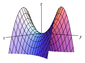
This is a graph of a hyperbolic paraboloid and at the origin we can see that if we move in along the \(y\)-axis the graph is increasing and if we move along the \(x\)-axis the graph is decreasing. So it is completely possible to have a graph both increasing and decreasing at a point depending upon the direction that we move. We should never expect that the function will behave in exactly the same way at a point as each variable changes.
The next interpretation was one of the standard interpretations in a Calculus I class. We know from a Calculus I class that \(f'\left( a \right)\) represents the slope of the tangent line to \(y = f\left( x \right)\) at \(x = a\). Well, \({f_x}\left( {a,b} \right)\) and \({f_y}\left( {a,b} \right)\) also represent the slopes of tangent lines. The difference here is the functions that they represent tangent lines to.
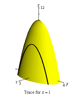
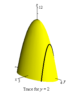
Partial derivatives are the slopes of traces. The partial derivative \({f_x}\left( {a,b} \right)\) is the slope of the trace of \(f\left( {x,y} \right)\) for the plane \(y = b\) at the point \(\left( {a,b} \right)\). Likewise the partial derivative \({f_y}\left( {a,b} \right)\) is the slope of the trace of \(f\left( {x,y} \right)\) for the plane \(x = a\) at the point \(\left( {a,b} \right)\).
We sketched the traces for the planes \(x = 1\) and \(y = 2\) in a previous section and these are the two traces for this point. For reference purposes here are the graphs of the traces.
Next, we’ll need the two partial derivatives so we can get the slopes.
\[{f_x}\left( {x,y} \right) = - 8x\hspace{0.5in}{f_y}\left( {x,y} \right) = - 2y\]To get the slopes all we need to do is evaluate the partial derivatives at the point in question.
\[{f_x}\left( {1,2} \right) = - 8\hspace{0.5in}{f_y}\left( {1,2} \right) = - 4\]So, the tangent line at \(\left( {1,2} \right)\) for the trace to \(z = 10 - 4{x^2} - {y^2}\) for the plane \(y = 2\) has a slope of -8. Also the tangent line at \(\left( {1,2} \right)\) for the trace to \(z = 10 - 4{x^2} - {y^2}\) for the plane \(x = 1\) has a slope of -4.
Finally, let’s briefly talk about getting the equations of the tangent line. Recall that the equation of a line in 3-D space is given by a vector equation. Also, to get the equation we need a point on the line and a vector that is parallel to the line.
The point is easy. Since we know the \(x\)-\(y\) coordinates of the point all we need to do is plug this into the equation to get the point. So, the point will be,
\[\left( {a,b,f\left( {a,b} \right)} \right)\]The parallel (or tangent) vector is also just as easy. We can write the equation of the surface as a vector function as follows,
\[\vec r\left( {x,y} \right) = \left\langle {x,y,z} \right\rangle = \left\langle {x,y,f\left( {x,y} \right)} \right\rangle \]We know that if we have a vector function of one variable we can get a tangent vector by differentiating the vector function. The same will hold true here. If we differentiate with respect to \(x\) we will get a tangent vector to traces for the plane \(y = b\) (i.e. for fixed \(y\)) and if we differentiate with respect to \(y\) we will get a tangent vector to traces for the plane \(x = a\) (or fixed \(x\)).
So, here is the tangent vector for traces with fixed \(y\).
\[{\vec r_x}\left( {x,y} \right) = \left\langle {1,0,{f_x}\left( {x,y} \right)} \right\rangle \]We differentiated each component with respect to \(x\). Therefore, the first component becomes a 1 and the second becomes a zero because we are treating \(y\) as a constant when we differentiate with respect to \(x\). The third component is just the partial derivative of the function with respect to \(x\).
For traces with fixed \(x\) the tangent vector is,
\[{\vec r_y}\left( {x,y} \right) = \left\langle {0,1,{f_y}\left( {x,y} \right)} \right\rangle \]The equation for the tangent line to traces with fixed \(y\) is then,
\[\vec r\left( t \right) = \left\langle {a,b,f\left( {a,b} \right)} \right\rangle + t\left\langle {1,0,{f_x}\left( {a,b} \right)} \right\rangle \]and the tangent line to traces with fixed \(x\) is,
\[\vec r\left( t \right) = \left\langle {a,b,f\left( {a,b} \right)} \right\rangle + t\left\langle {0,1,{f_y}\left( {a,b} \right)} \right\rangle \]There really isn’t all that much to do with these other than plugging the values and function into the formulas above. We’ve already computed the derivatives and their values at \(\left( {1,2} \right)\) in the previous example and the point on each trace is,
\[\left( {1,2,f\left( {1,2} \right)} \right) = \left( {1,2,2} \right)\]Here is the equation of the tangent line to the trace for the plane \(y = 2\).
\[\vec r\left( t \right) = \left\langle {1,2,2} \right\rangle + t\left\langle {1,0, - 8} \right\rangle = \left\langle {1 + t,2,2 - 8t} \right\rangle \]Here is the equation of the tangent line to the trace for the plane \(x = 1\).
\[\vec r\left( t \right) = \left\langle {1,2,2} \right\rangle + t\left\langle {0,1, - 4} \right\rangle = \left\langle {1,2 + t,2 - 4t} \right\rangle \]