Section 15.1 : Double Integrals
Before starting on double integrals let’s do a quick review of the definition of definite integrals for functions of single variables. First, when working with the integral,
\[\int_{{\,a}}^{{\,b}}{{f\left( x \right)\,dx}}\]we think of \(x\)’s as coming from the interval \(a \le x \le b\). For these integrals we can say that we are integrating over the interval \(a \le x \le b\). Note that this does assume that \(a < b\), however, if we have \(b < a\) then we can just use the interval \(b \le x \le a\).
Now, when we derived the definition of the definite integral we first thought of this as an area problem. We first asked what the area under the curve was and to do this we broke up the interval \(a \le x \le b\) into \(n\) subintervals of width \(\Delta x\) and choose a point, \(x_i^*\), from each interval as shown below,
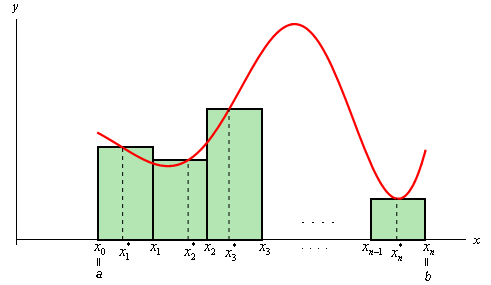
Each of the rectangles has height of \(f\left( {x_i^*} \right)\) and we could then use the area of each of these rectangles to approximate the area as follows.
\[A \approx f\left( {x_1^*} \right)\Delta x + f\left( {x_2^*} \right)\Delta x + \cdots + f\left( {x_i^*} \right)\Delta x + \cdots + f\left( {x_n^*} \right)\Delta x\]To get the exact area we then took the limit as \(n\) goes to infinity and this was also the definition of the definite integral.
\[\int_{{\,a}}^{{\,b}}{{f\left( x \right)\,dx}} = \mathop {\lim }\limits_{n \to \infty } \sum\limits_{i = 1}^n {f\left( {x_i^*} \right)\Delta x} \]In this section we want to integrate a function of two variables,\(f\left( {x,y} \right)\). With functions of one variable we integrated over an interval (i.e. a one-dimensional space) and so it makes some sense then that when integrating a function of two variables we will integrate over a region of \({\mathbb{R}^2}\)(two-dimensional space).
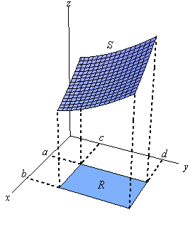
We will start out by assuming that the region in \({\mathbb{R}^2}\) is a rectangle which we will denote as follows,
\[R = \left[ {a,b} \right] \times \left[ {c,d} \right]\]This means that the ranges for \(x\) and \(y\) are \(a \le x \le b\) and \(c \le y \le d\).
Also, we will initially assume that \(f\left( {x,y} \right) \ge 0\) although this doesn’t really have to be the case. Let’s start out with the graph of the surface \(S\) given by graphing \(f\left( {x,y} \right)\) over the rectangle \(R\).
Now, just like with functions of one variable let’s not worry about integrals quite yet. Let’s first ask what the volume of the region under \(S\) (and above the xy-plane of course) is.
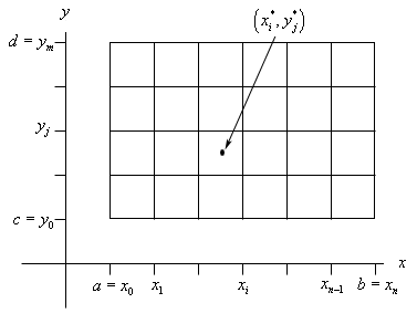
We will approximate the volume much as we approximated the area above. We will first divide up \(a \le x \le b\) into \(n\) subintervals and divide up \(c \le y \le d\) into \(m\) subintervals. This will divide up \(R\) into a series of smaller rectangles and from each of these we will choose a point \(\left( {x_i^*,y_j^*} \right)\). Here is a sketch of this set up.
Now, over each of these smaller rectangles we will construct a box whose height is given by \(f\left( {x_i^*,y_j^*} \right)\). Here is a sketch of that.
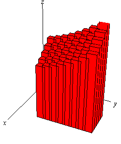
Each of the rectangles has a base area of \(\Delta {\kern 1pt} A\) and a height of \(f\left( {x_i^*,y_j^*} \right)\) so the volume of each of these boxes is \(f\left( {x_i^*,y_j^*} \right)\,\Delta {\kern 1pt} A\). The volume under the surface \(S\) is then approximately,
\[V \approx \sum\limits_{i = 1}^n {\sum\limits_{j = 1}^m {f\left( {x_i^*,y_j^*} \right)\,\Delta {\kern 1pt} A} } \]We will have a double sum since we will need to add up volumes in both the \(x\) and \(y\) directions.
To get a better estimation of the volume we will take \(n\) and \(m\) larger and larger and to get the exact volume we will need to take the limit as both \(n\) and \(m\) go to infinity. In other words,
\[V = \mathop {\lim }\limits_{n,\,\,m \to \infty } \sum\limits_{i = 1}^n {\sum\limits_{j = 1}^m {f\left( {x_i^*,y_j^*} \right)\,\Delta {\kern 1pt} A} } \]Now, this should look familiar. This looks a lot like the definition of the integral of a function of single variable. In fact, this is also the definition of a double integral, or more exactly an integral of a function of two variables over a rectangle.
Here is the official definition of a double integral of a function of two variables over a rectangular region \(R\) as well as the notation that we’ll use for it.
\[\iint\limits_{R}{{f\left( {x,y} \right)\,dA}} = \mathop {\lim }\limits_{n,\,\,m \to \infty } \sum\limits_{i = 1}^n {\sum\limits_{j = 1}^m {f\left( {x_i^*,y_j^*} \right)\,\Delta {\kern 1pt} A} } \]Note the similarities and differences in the notation to single integrals. We have two integrals to denote the fact that we are dealing with a two dimensional region and we have a differential here as well. Note that the differential is \(dA\) instead of the \(dx\) and \(dy\) that we’re used to seeing. Note as well that we don’t have limits on the integrals in this notation. Instead we have the \(R\) written below the two integrals to denote the region that we are integrating over.
As indicated above one interpretation of the double integral of \(f\left( {x,y} \right)\) over the rectangle \(R\) is the volume under the function \(f\left( {x,y} \right)\) (and above the xy-plane). Or,
We can use this double sum in the definition to estimate the value of a double integral if we need to. We can do this by choosing \(\left( {x_i^*,y_j^*} \right)\) to be the midpoint of each rectangle. When we do this we usually denote the point as \(\left( {{{\overline{x}}_i},{{\overline{y}}_j}} \right)\). This leads to the Midpoint Rule,
\[\iint\limits_{R}{{f\left( {x,y} \right)\,dA}} \approx \sum\limits_{i = 1}^n {\sum\limits_{j = 1}^m {f\left( {{{\overline{x}}_i},{{\overline{y}}_j}} \right)\,\Delta {\kern 1pt} A} } \]In the next section we start looking at how to actually compute double integrals.