Section 3.1 : Graphing
In this section we need to review some of the basic ideas in graphing. It is assumed that you’ve seen some graphing to this point and so we aren’t going to go into great depth here. We will only be reviewing some of the basic ideas.
We will start off with the Rectangular or Cartesian coordinate system. This is just the standard axis system that we use when sketching our graphs. Here is the Cartesian coordinate system with a few points plotted.
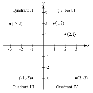
The horizontal and vertical axes, typically called the \(x\)-axis and the \(y\)-axis respectively, divide the coordinate system up into quadrants as shown above. In each quadrant we have the following signs for \(x\) and \(y\).
| Quadrant I | \(x > 0\), or \(x\) positive | \(y > 0\), or \(y\) positive |
| Quadrant II | \(x < 0\), or \(x\) negative | \(y > 0\), or \(y\) positive |
| Quadrant III | \(x < 0\), or \(x\) negative | \(y < 0\), or \(y\) negative |
| Quadrant IV | \(x > 0\), or \(x\) positive | \(y < 0\), or \(y\) negative |
Each point in the coordinate system is defined by an ordered pair of the form \(\left( {x,y} \right)\). The first number listed is the \(x\)-coordinate of the point and the second number listed is the \(y\)-coordinate of the point. The ordered pair for any given point, \(\left( {x,y} \right)\), is called the coordinates for the point.
The point where the two axes cross is called the origin and has the coordinates \(\left( {0,0} \right)\).
Note as well that the order of the coordinates is important. For example, the point \(\left( {2,1} \right)\) is the point that is two units to the right of the origin and then 1 unit up, while the point \(\left( {1,2} \right)\) is the point that is 1 unit to the right of the origin and then 2 units up.
We now need to discuss graphing an equation. The first question that we should ask is what exactly is a graph of an equation? A graph is the set of all the ordered pairs whose coordinates satisfy the equation.
For instance, the point \(\left( {2, - 3} \right)\) is a point on the graph of \(y = {\left( {x - 1} \right)^2} - 4\) while \(\left( {1,5} \right)\) isn’t on the graph. How do we tell this? All we need to do is take the coordinates of the point and plug them into the equation to see if they satisfy the equation. Let’s do that for both to verify the claims made above.
\(\left( {2, - 3} \right)\):In this case we have \(x = 2\) and \(y = - 3\) so plugging in gives,
\[\begin{align*} - 3 & \mathop = \limits^? {\left( {2 - 1} \right)^2} - 4\\ - 3 & \mathop = \limits^? {\left( 1 \right)^2} - 4\\ - 3 & = - 3\hspace{0.25in}{\mbox{OK}}\end{align*}\]So, the coordinates of this point satisfies the equation and so it is a point on the graph.
\(\left( {1,5} \right)\):Here we have \(x = 1\) and \(y = 5\). Plugging these in gives,
\[\begin{align*}5 & \mathop = \limits^? {\left( {1 - 1} \right)^2} - 4\\ 5 & \mathop = \limits^? {\left( 0 \right)^2} - 4\\ 5 & \ne - 4\hspace{0.25in}{\mbox{NOT OK}}\end{align*}\]The coordinates of this point do NOT satisfy the equation and so this point isn’t on the graph.
Now, how do we sketch the graph of an equation? Of course, the answer to this depends on just how much you know about the equation to start off with. For instance, if you know that the equation is a line or a circle we’ve got simple ways to determine the graph in these cases. There are also many other kinds of equations that we can usually get the graph from the equation without a lot of work. We will see many of these in the next chapter.
However, let’s suppose that we don’t know ahead of time just what the equation is or any of the ways to quickly sketch the graph. In these cases we will need to recall that the graph is simply all the points that satisfy the equation. So, all we can do is plot points. We will pick values of \(x\), compute \(y\) from the equation and then plot the ordered pair given by these two values.
How, do we determine which values of \(x\) to choose? Unfortunately, the answer there is we guess. We pick some values and see what we get for a graph. If it looks like we’ve got a pretty good sketch we stop. If not we pick some more. Knowing the values of \(x\) to choose is really something that we can only get with experience and some knowledge of what the graph of the equation will probably look like. Hopefully, by the end of this course you will have gained some of this knowledge.
Let’s take a quick look at a graph.
Now, this is a parabola and after the next chapter you will be able to quickly graph this without much effort. However, we haven’t gotten that far yet and so we will need to choose some values of \(x\), plug them in and compute the \(y\) values.
As mentioned earlier, it helps to have an idea of what this graph is liable to look like when picking values of \(x\). So, don’t worry at this point why we chose the values that we did. After the next chapter you would also be able to choose these values of \(x\).
Here is a table of values for this equation.
| \(x\) | \(y\) | \(\left( {x,y} \right)\) |
|---|---|---|
| -2 | 5 | \(\left( { - 2,5} \right)\) |
| -1 | 0 | \(\left( { - 1,0} \right)\) |
| 0 | -3 | \(\left( {0, - 3} \right)\) |
| 1 | -4 | \(\left( {1, - 4} \right)\) |
| 2 | -3 | \(\left( {2, - 3} \right)\) |
| 3 | 0 | \(\left( {3,0} \right)\) |
| 4 | 5 | \(\left( {4,5} \right)\) |
Let’s verify the first one and we’ll leave the rest to you to verify. For the first one we simply plug \(x = - 2\) into the equation and compute \(y\).
\[\begin{align*}y & = {\left( { - 2 - 1} \right)^2} - 4\\ & = {\left( { - 3} \right)^2} - 4\\ & = 9 - 4\\ & = 5\end{align*}\]Here is the graph of this equation.
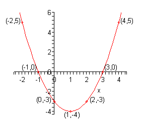
Notice that when we set up the axis system in this example, we only set up as much as we needed. For example, since we didn’t go past -2 with our computations we didn’t go much past that with our axis system.
Also, notice that we used a different scale on each of the axes. With the horizontal axis we incremented by 1’s while on the vertical axis we incremented by 2. This will often be done in order to make the sketching easier.
The final topic that we want to discuss in this section is that of intercepts. Notice that the graph in the above example crosses the \(x\)-axis in two places and the \(y\)-axis in one place. All three of these points are called intercepts. We can, and often will be, more specific however.
We often will want to know if an intercept crosses the \(x\) or \(y\)-axis specifically. So, if an intercept crosses the \(x\)-axis we will call it an \(x\)-intercept. Likewise, if an intercept crosses the \(y\)-axis we will call it a \(y\)-intercept.
Now, since the \(x\)-intercept crosses \(x\)-axis then the \(y\) coordinates of the \(x\)-intercept(s) will be zero. Also, the \(x\) coordinate of the \(y\)-intercept will be zero since these points cross the \(y\)-axis. These facts give us a way to determine the intercepts for an equation. To find the \(x\)-intercepts for an equation all that we need to do is set \(y = 0\) and solve for \(x\). Likewise, to find the \(y\)-intercepts for an equation we simply need to set \(x = 0\) and solve for \(y\).
Let’s take a quick look at an example.
- \(y = {x^2} + x - 6\)
- \(y = {x^2} + 2\)
- \(y = {\left( {x + 1} \right)^2}\)
As verification for each of these we will also sketch the graph of each function. We will leave the details of the sketching to you to verify. Also, these are all parabolas and as mentioned earlier we will be looking at these in detail in the next chapter.
a \(y = {x^2} + x - 6\) Show Solution
Let’s first find the \(y\)-intercept(s). Again, we do this by setting \(x = 0\) and solving for \(y\). This is usually the easier of the two. So, let’s find the \(y\)-intercept(s).
\[y = {\left( 0 \right)^2} + 0 - 6 = - 6\]So, there is a single \(y\)-intercept : \(\left( {0, - 6} \right)\).
The work for the \(x\)-intercept(s) is almost identical except in this case we set \(y = 0\) and solve for \(x\). Here is that work.
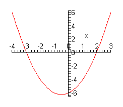
\[\begin{align*}0 & = {x^2} + x - 6\\ 0 & = \left( {x + 3} \right)\left( {x - 2} \right)\hspace{0.25in} \Rightarrow \hspace{0.25in}x = - 3,\,\,\,x = 2\end{align*}\]For this equation there are two \(x\)-intercepts : \(\left( { - 3,0} \right)\) and \(\left( {2,0} \right)\). Oh, and you do remember how to solve quadratic equations right?
For verification purposes here is sketch of the graph for this equation.
b \(y = {x^2} + 2\) Show Solution
First, the \(y\)-intercepts.
\[y = {\left( 0 \right)^2} + 2 = 2\hspace{0.25in} \Rightarrow \hspace{0.25in}\left( {0,2} \right)\]So, we’ve got a single \(y\)-intercepts. Now, the \(x\)-intercept(s).
\[\begin{align*}0 & = {x^2} + 2\\ - 2 & = {x^2}\hspace{0.25in} \Rightarrow \hspace{0.25in}x = \pm \sqrt 2 \,i\end{align*}\]Okay, we got complex solutions from this equation. What this means is that we will not have any \(x\)-intercepts. Note that it is perfectly acceptable for this to happen so don’t worry about it when it does happen.
Here is the graph for this equation.
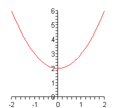
Sure enough, it doesn’t cross the \(x\)-axis.
c \(y = {\left( {x + 1} \right)^2}\) Show Solution
Here is the \(y\)-intercept work for this equation.
\[y = {\left( {0 + 1} \right)^2} = 1\hspace{0.25in} \Rightarrow \hspace{0.25in}\left( {0,1} \right)\]Now the \(x\)-intercept work.
\[0 = {\left( {x + 1} \right)^2}\hspace{0.25in} \Rightarrow \hspace{0.25in}x = - 1\hspace{0.25in} \Rightarrow \hspace{0.25in}\left( { - 1,0} \right)\]In this case we have a single \(x\)-intercept.
Here is a sketch of the graph for this equation.
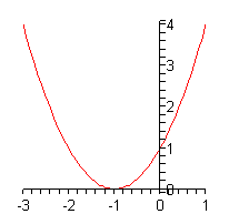
Now, notice that in this case the graph doesn’t actually cross the \(x\)-axis at \(x = - 1\). This point is still called an \(x\)-intercept however.
We should make one final comment before leaving this section. In the previous set of examples all the equations were quadratic equations. This was done only because they exhibited the range of behaviors that we were looking for and we would be able to do the work as well. You should not walk away from this discussion of intercepts with the idea that they will only occur for quadratic equations. They can, and do, occur for many different equations.