Section 4.6 : The Shape of a Graph, Part II
In the previous section we saw how we could use the first derivative of a function to get some information about the graph of a function. In this section we are going to look at the information that the second derivative of a function can give us a about the graph of a function.
Before we do this we will need a couple of definitions out of the way. The main concept that we’ll be discussing in this section is concavity. Concavity is easiest to see with a graph (we’ll give the mathematical definition in a bit).
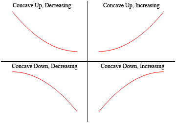
So, a function is concave up if it “opens” up and the function is concave down if it “opens” down. Notice as well that concavity has nothing to do with increasing or decreasing. A function can be concave up and either increasing or decreasing. Similarly, a function can be concave down and either increasing or decreasing.
It’s probably not the best way to define concavity by saying which way it “opens” since this is a somewhat nebulous definition. Here is the mathematical definition of concavity.
Definition 1
Given the function \(f\left( x \right)\) then
- \(f\left( x \right)\) is concave up on an interval \(I\) if all of the tangents to the curve on \(I\) are below the graph of \(f\left( x \right)\).
- \(f\left( x \right)\) is concave down on an interval \(I\) if all of the tangents to the curve on \(I\) are above the graph of \(f\left( x \right)\).
To show that the graphs above do in fact have concavity claimed above here is the graph again (blown up a little to make things clearer).
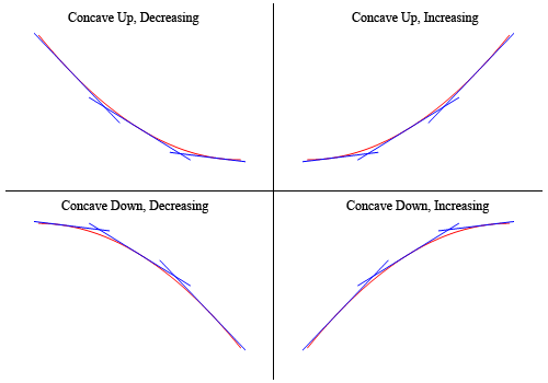
So, as you can see, in the two upper graphs all of the tangent lines sketched in are all below the graph of the function and these are concave up. In the lower two graphs all the tangent lines are above the graph of the function and these are concave down.
Again, notice that concavity and the increasing/decreasing aspect of the function is completely separate and do not have anything to do with each other. This is important to note because students often mix these two up and use information about one to get information about the other.
There’s one more definition that we need to get out of the way.
Definition 2
A point \(x = c\) is called an inflection point if the function is continuous at the point and the concavity of the graph changes at that point.
Now that we have all the concavity definitions out of the way we need to bring the second derivative into the mix. We did after all start off this section saying we were going to be using the second derivative to get information about the graph. The following fact relates the second derivative of a function to its concavity. The proof of this fact is in the Proofs From Derivative Applications section of the Extras chapter.
Fact
Given the function \(f\left( x \right)\) then,
- If \(f''\left( x \right) > 0\) for all \(x\) in some interval \(I\) then \(f\left( x \right)\) is concave up on \(I\).
- If \(f''\left( x \right) < 0\) for all \(x\) in some interval \(I\) then \(f\left( x \right)\) is concave down on \(I\).
So, what this fact tells us is that the inflection points will be all the points where the second derivative changes sign. We saw in the previous chapter that a function may change signs if it is either zero or does not exist. Note that we were working with the first derivative in the previous section but the fact that a function possibly changing signs where it is zero or doesn’t exist has nothing to do with the first derivative. It is simply a fact that applies to all functions regardless of whether they are derivatives or not.
This in turn tells us that a list of possible inflection points will be those points where the second derivative is zero or doesn’t exist, as these are the only points where the second derivative might change sign.
Be careful however to not make the assumption that just because the second derivative is zero or doesn’t exist that the point will be an inflection point. We will only know that it is an inflection point once we determine the concavity on both sides of it. It will only be an inflection point if the concavity is different on both sides of the point.
Now that we know about concavity we can use this information as well as the increasing/decreasing information from the previous section to get a pretty good idea of what a graph should look like. Let’s take a look at an example of that.
Okay, we are going to need the first two derivatives so let’s get those first.
\[\begin{align*}h'\left( x \right) & = 15{x^4} - 15{x^2} = 15{x^2}\left( {x - 1} \right)\left( {x + 1} \right)\\ h''\left( x \right) & = 60{x^3} - 30x = 30x\left( {2{x^2} - 1} \right)\end{align*}\]Let’s start with the increasing/decreasing information since we should be fairly comfortable with that after the last section.
There are three critical points for this function : \(x = - 1\), \(x = 0\), and \(x = 1\). Below is the number line for the increasing/decreasing information.
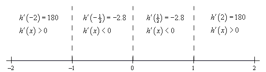
So, it looks like we’ve got the following intervals of increasing and decreasing.
\[\begin{align*}{\mbox{Increasing : }} & - \infty < x < - 1{\mbox{ and }}1 < x < \infty \\ {\mbox{Decreasing : }} & - 1 < x < 0,\,\,\,0 < x < 1\end{align*}\]Note that from the first derivative test we can also say that \(x = - 1\) is a relative maximum and that \(x = 1\) is a relative minimum. Also \(x = 0\) is neither a relative minimum or maximum.
Now let’s get the intervals where the function is concave up and concave down. If you think about it this process is almost identical to the process we use to identify the intervals of increasing and decreasing. This only difference is that we will be using the second derivative instead of the first derivative.
The first thing that we need to do is identify the possible inflection points. These will be where the second derivative is zero or doesn’t exist. The second derivative in this case is a polynomial and so will exist everywhere. It will be zero at the following points.
\[x = 0,\,\,x = \pm \frac{1}{{\sqrt 2 }} = \pm \,0.7071\]As with the increasing and decreasing part we can draw a number line up and use these points to divide the number line into regions. In these regions we know that the second derivative will always have the same sign since these three points are the only places where the function may change sign. Therefore, all that we need to do is pick a point from each region and plug it into the second derivative. The second derivative will then have that sign in the whole region from which the point came from
Here is the number line for this second derivative.
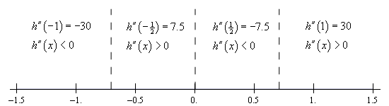
So, it looks like we’ve got the following intervals of concavity.
\[\begin{align*}{\mbox{Concave Up : }} & - \frac{1}{{\sqrt 2 }} < x < 0{\mbox{ and }}\frac{1}{{\sqrt 2 }} < x < \infty \\ {\mbox{Concave Down : }} & - \infty < x < - \frac{1}{{\sqrt 2 }}{\mbox{ and }}0 < x < \frac{1}{{\sqrt 2 }}\end{align*}\]This also means that
\[x = 0,\,\,x = \pm \frac{1}{{\sqrt 2 }} = \pm 0.7071\]are all inflection points.
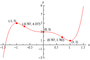
All this information can be a little overwhelming when going to sketch the graph. The first thing that we should do is get some starting points. The critical points and inflection points are good starting points. So, first graph these points.
From this point there are several ways to proceed with sketching the graph. The way that we find to be the easiest (although you may not and that is perfectly fine….) is to start with the increasing/decreasing information and start sketching the graph from just that information as we did in the previous section. However, unlike the previous section, this time as we draw an increasing or decreasing portion of the curve we will also pay attention to the concavity of the curve as we are doing this.
So, if we start with \(x < - 1\) we know that we have an increasing function. At the same time, we know that we also have to be concave down in this range. So, we can start off with sketching an increasing curve that has is also concave down until we reach \(x = - 1\).
At this point the graph starts to decrease and will continue to decrease until we hit \(x = 1\). However, as we decrease the concavity needs to switch to concave up at \(x \approx - 0.707\) and then switch back to concave down at \(x = 0\) with a final switch to concave up at \(x \approx 0.707\).
Once we hit \(x = 1\) the graph starts to increase and is still concave up and both of these behaviors continue for the rest of the graph.
Putting all this information together will give us the following graph of the function.
We can use the previous example to illustrate another way to classify some of the critical points of a function as relative maximums or relative minimums.
Notice that \(x = - 1\) is a relative maximum and that the function is concave down at this point. This means that \(f''\left( { - 1} \right)\) must be negative. Likewise, \(x = 1\) is a relative minimum and the function is concave up at this point. This means that \(f''\left( 1 \right)\) must be positive.
As we’ll see in a bit we will need to be very careful with \(x = 0\). In this case the second derivative is zero, but that will not actually mean that \(x = 0\) is not a relative minimum or maximum. We’ll see some examples of this in a bit, but we need to get some other information taken care of first.
It is also important to note here that all of the critical points in this example were critical points in which the first derivative was zero and this is required for this to work. We will not be able to use this test on critical points where the derivative doesn’t exist.
Here is the test that can be used to classify some of the critical points of a function. The proof of this test is in the Proofs of Derivative Applications section of the Extras chapter.
Second Derivative Test
Suppose that \(x = c\) is a critical point of \(f\left( x \right)\) such that \(f'\left( c \right) = 0\) and that \(f''\left( x \right)\) is continuous in a region around \(x = c\). Then,
- If \(f''\left( c \right) < 0\) then \(x = c\) is a relative maximum.
- If \(f''\left( c \right) > 0\) then \(x = c\) is a relative minimum.
- If \(f''\left( c \right) = 0\) then \(x = c\) can be a relative maximum, relative minimum or neither.
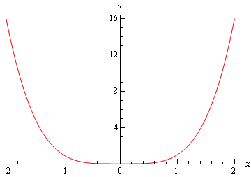
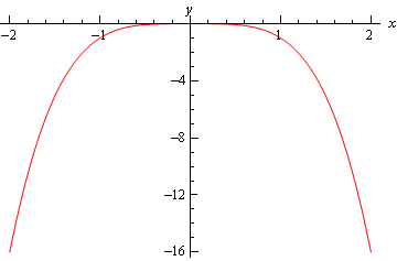
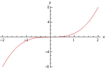
The third part of the second derivative test is important to notice. If the second derivative is zero then the critical point can be anything. Below are the graphs of three functions all of which have a critical point at \(x = 0\), the second derivative of all of the functions is zero at \(x = 0\) and yet all three possibilities are exhibited.
The first is the graph of \(f\left( x \right) = {x^4}\). This graph has a relative minimum at \(x = 0\).
Next is the graph of \(f\left( x \right) = - {x^4}\) which has a relative maximum at \(x = 0\).
Finally, there is the graph of \(f\left( x \right) = {x^3}\) and this graph had neither a relative minimum or a relative maximum at \(x = 0\).
So, we can see that we have to be careful if we fall into the third case. For those times when we do fall into this case we will have to resort to other methods of classifying the critical point. This is usually done with the first derivative test.
Let’s go back and take a look at the critical points from the first example and use the Second Derivative Test on them, if possible.
Note that all we’re doing here is verifying the results from the first example. The second derivative is,
\[h''\left( x \right) = 60{x^3} - 30x\]The three critical points (\(x = - 1\), \(x = 0\), and \(x = 1\)) of this function are all critical points where the first derivative is zero so we know that we at least have a chance that the Second Derivative Test will work. The value of the second derivative for each of these are,
\[h''\left( { - 1} \right) = - 30\hspace{0.5in}h''\left( 0 \right) = 0\hspace{0.5in}h''\left( 1 \right) = 30\]The second derivative at \(x = - 1\) is negative so by the Second Derivative Test this critical point this is a relative maximum as we saw in the first example. The second derivative at \(x = 1\) is positive and so we have a relative minimum here by the Second Derivative Test as we also saw in the first example.
In the case of \(x = 0\) the second derivative is zero and so we can’t use the Second Derivative Test to classify this critical point. Note however, that we do know from the First Derivative Test we used in the first example that in this case the critical point is not a relative extrema.
Let’s work one more example.
We’ll need the first and second derivatives to get us started. We’ll leave it to you to verify these derivatives but be aware that we did a little simplification after taking each derivative.
\[f'\left( t \right) = \frac{{18 - 5t}}{{3{{\left( {6 - t} \right)}^{\frac{1}{3}}}}}\hspace{0.5in}f''\left( t \right) = \frac{{10t - 72}}{{9{{\left( {6 - t} \right)}^{\frac{4}{3}}}}}\]The critical points are,
\[t = \frac{{18}}{5} = 3.6\hspace{0.5in}t = 6\]Notice as well that we won’t be able to use the second derivative test on \(t = 6\) to classify this critical point since the derivative doesn’t exist at this point. To classify this, we’ll need the increasing/decreasing information that we’ll get to sketch the graph.
We can however, use the Second Derivative Test to classify the other critical point so let’s do that before we proceed with the sketching work. Here is the value of the second derivative at \(t = 3.6\).
\[f''\left( {3.6} \right) = - 1.245 < 0\]So, according to the second derivative test \(t = 3.6\) is a relative maximum.
Now let’s proceed with the work to get the sketch of the graph and notice that once we have the increasing/decreasing information we’ll be able to classify \(t = 6\).
Here is the number line for the first derivative.
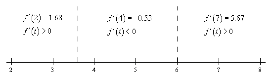
So, according to the first derivative test we can verify that \(t = 3.6\) is in fact a relative maximum. We can also see that \(t = 6\) is a relative minimum.
Be careful not to assume that a critical point that can’t be used in the second derivative test won’t be a relative extrema. We’ve clearly seen now both with this example and in the discussion after we have the test that just because we can’t use the Second Derivative Test or the Second Derivative Test doesn’t tell us anything about a critical point doesn’t mean that the critical point will not be a relative extrema. This is a common mistake that many students make so be careful when using the Second Derivative Test.
Okay, let’s finish the problem out. We will need the list of possible inflection points. These are,
\[t = 6\hspace{0.5in}t = \frac{{72}}{{10}} = 7.2\]Here is the number line for the second derivative. Note that we will need this to see if the two points above are in fact inflection points.
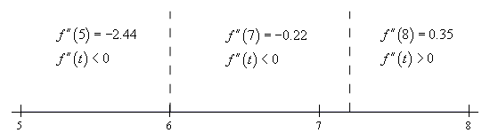
So, the concavity only changes at \(t = 7.2\) and so this is the only inflection point for this function.
Here is the sketch of the graph.
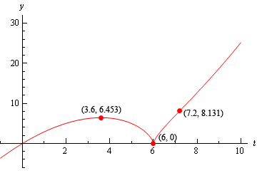
The change of concavity at \(t = 7.2\) is hard to see, but it is there it’s just a very subtle change in concavity.