Section 10.1 : Sequences
Let’s start off this section with a discussion of just what a sequence is. A sequence is nothing more than a list of numbers written in a specific order. The list may or may not have an infinite number of terms in it although we will be dealing exclusively with infinite sequences in this class. General sequence terms are denoted as follows,
\[\begin{align*}& {a_1} - {\mbox{first term}}\\ & {a_2} - {\mbox{second term}}\\ & \hspace{0.75in} \vdots \\ & {a_n} - {n^{th}}{\mbox{ term}}\\ & {a_{n + 1}} - {\left( {n + 1} \right)^{{\mbox{st}}}}{\mbox{ term}}\\ & \hspace{0.75in} \vdots \end{align*}\]Because we will be dealing with infinite sequences each term in the sequence will be followed by another term as noted above. In the notation above we need to be very careful with the subscripts. The subscript of \(n + 1\) denotes the next term in the sequence and NOT one plus the \(n^{\mbox{th}}\) term! In other words,
\[{a_{n + 1}} \ne {a_n} + 1\]so be very careful when writing subscripts to make sure that the “+1” doesn’t migrate out of the subscript! This is an easy mistake to make when you first start dealing with this kind of thing.
There is a variety of ways of denoting a sequence. Each of the following are equivalent ways of denoting a sequence.
\[\left\{ {{a_1},{a_2}, \ldots ,{a_n},{a_{n + 1}}, \ldots } \right\}\hspace{0.5in}\left\{ {{a_n}} \right\}\hspace{0.5in}\left\{ {{a_n}} \right\}_{n = 1}^\infty \]In the second and third notations above an is usually given by a formula.
A couple of notes are now in order about these notations. First, note the difference between the second and third notations above. If the starting point is not important or is implied in some way by the problem it is often not written down as we did in the third notation. Next, we used a starting point of \(n = 1\) in the third notation only so we could write one down. There is absolutely no reason to believe that a sequence will start at \(n = 1\). A sequence will start whereever it needs to start.
Let’s take a look at a couple of sequences.
- \(\displaystyle \left\{ {\frac{{n + 1}}{{{n^2}}}} \right\}_{n = 1}^\infty \)
- \(\displaystyle \left\{ {\frac{{{{\left( { - 1} \right)}^{n + 1}}}}{{{2^n}}}} \right\}_{n = 0}^\infty \)
- \(\left\{ {{b_n}} \right\}_{n = 1}^\infty \), where \({b_n} = {n^{th}}{\mbox{ digit of }}\pi \)
To get the first few sequence terms here all we need to do is plug in values of \(n\) into the formula given and we’ll get the sequence terms.
\[\left\{ {\frac{{n + 1}}{{{n^2}}}} \right\}_{n = 1}^\infty = \left\{ {\underbrace 2_{n = 1},\underbrace {\frac{3}{4}}_{n = 2},\underbrace {\frac{4}{9}}_{n = 3},\underbrace {\frac{5}{{16}}}_{n = 4},\underbrace {\frac{6}{{25}}}_{n = 5}, \ldots } \right\}\]Note the inclusion of the “…” at the end! This is an important piece of notation as it is the only thing that tells us that the sequence continues on and doesn’t terminate at the last term.
b \(\displaystyle \left\{ {\frac{{{{\left( { - 1} \right)}^{n + 1}}}}{{{2^n}}}} \right\}_{n = 0}^\infty \) Show Solution
This one is similar to the first one. The main difference is that this sequence doesn’t start at \(n = 1\).
\[\left\{ {\frac{{{{\left( { - 1} \right)}^{n + 1}}}}{{{2^n}}}} \right\}_{n = 0}^\infty = \left\{ { - 1,\frac{1}{2}, - \frac{1}{4},\frac{1}{8}, - \frac{1}{{16}}, \ldots } \right\}\]Note that the terms in this sequence alternate in signs. Sequences of this kind are sometimes called alternating sequences.
c \(\left\{ {{b_n}} \right\}_{n = 1}^\infty \), where \({b_n} = {n^{th}}{\mbox{ digit of }}\pi \) Show Solution
This sequence is different from the first two in the sense that it doesn’t have a specific formula for each term. However, it does tell us what each term should be. Each term should be the nth digit of \(\pi\). So we know that \(\pi = 3.14159265359 \ldots \)
The sequence is then,
\[\left\{ {3,1,4,1,5,9,2,6,5,3,5, \ldots } \right\}\]In the first two parts of the previous example note that we were really treating the formulas as functions that can only have integers plugged into them. Or,
\[f\left( n \right) = \frac{{n + 1}}{{{n^2}}}\hspace{0.5in}\hspace{0.25in}g\left( n \right) = \frac{{{{\left( { - 1} \right)}^{n + 1}}}}{{{2^n}}}\]This is an important idea in the study of sequences (and series). Treating the sequence terms as function evaluations will allow us to do many things with sequences that we couldn’t do otherwise. Before delving further into this idea however we need to get a couple more ideas out of the way.
First, we want to think about “graphing” a sequence. To graph the sequence \(\left\{ {{a_n}} \right\}\) we plot the points \(\left( {n,{a_n}} \right)\) as \(n\) ranges over all possible values on a graph. For instance, let’s graph the sequence \(\left\{ {\frac{{n + 1}}{{{n^2}}}} \right\}_{n = 1}^\infty \). The first few points on the graph are,
\[\left( {1,2} \right),\,\,\left( {2,\frac{3}{4}} \right),\,\,\left( {3,\frac{4}{9}} \right),\,\,\left( {4,\frac{5}{{16}}} \right),\,\,\left( {5,\frac{6}{{25}}} \right),\,\, \ldots \]The graph, for the first 30 terms of the sequence, is then,
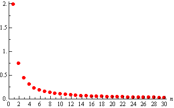
This graph leads us to an important idea about sequences. Notice that as \(n\) increases the sequence terms in our sequence, in this case, get closer and closer to zero. We then say that zero is the limit (or sometimes the limiting value) of the sequence and write,
\[\mathop {\lim }\limits_{n \to \infty } {a_n} = \mathop {\lim }\limits_{n \to \infty } \frac{{n + 1}}{{{n^2}}} = 0\]This notation should look familiar to you. It is the same notation we used when we talked about the limit of a function. In fact, if you recall, we said earlier that we could think of sequences as functions in some way and so this notation shouldn’t be too surprising.
Using the ideas that we developed for limits of functions we can write down the following working definition for limits of sequences.
Working Definition of Limit
- We say that
\[\mathop {\lim }\limits_{n \to \infty } {a_n} = L\]
if we can make an as close to \(L\) as we want for all sufficiently large \(n\). In other words, the value of the \({a_n}\)’s approach \(L\) as \(n\) approaches infinity.
- We say that
\[\mathop {\lim }\limits_{n \to \infty } {a_n} = \infty \]
if we can make an as large as we want for all sufficiently large \(n\). Again, in other words, the value of the \({a_n}\)’s get larger and larger without bound as \(n\) approaches infinity.
- We say that
\[\mathop {\lim }\limits_{n \to \infty } {a_n} = - \infty \]
if we can make an as large and negative as we want for all sufficiently large \(n\). Again, in other words, the value of the \({a_n}\)’s are negative and get larger and larger without bound as \(n\) approaches infinity.
The working definitions of the various sequence limits are nice in that they help us to visualize what the limit actually is. Just like with limits of functions however, there is also a precise definition for each of these limits. Let’s give those before proceeding
Precise Definition of Limit
- We say that \(\mathop {\lim }\limits_{n \to \infty } {a_n} = L\) if for every number \(\varepsilon > 0\) there is an integer \(N\) such that \[\left| {{a_n} - L} \right| < \varepsilon \hspace{0.5in}{\mbox{whenever}}\hspace{0.5in}n > N\]
- We say that \(\mathop {\lim }\limits_{n \to \infty } {a_n} = \infty \) if for every number \(M > 0\) there is an integer \(N\) such that \[{a_n} > M\hspace{0.5in}\,\,\,\,\,{\mbox{whenever}}\hspace{0.5in}n > N\]
- We say that \(\mathop {\lim }\limits_{n \to \infty } {a_n} = - \infty \) if for every number \(M < 0\) there is an integer \(N\) such that \[{a_n} < M\hspace{0.5in}\,\,\,\,\,{\mbox{whenever}}\hspace{0.5in}n > N\]
We won’t be using the precise definition often, but it will show up occasionally.
Note that both definitions tell us that in order for a limit to exist and have a finite value all the sequence terms must be getting closer and closer to that finite value as \(n\) increases.
Now that we have the definitions of the limit of sequences out of the way we have a bit of terminology that we need to look at. If \(\mathop {\lim }\limits_{n \to \infty } {a_n}\) exists and is finite we say that the sequence is convergent. If \(\mathop {\lim }\limits_{n \to \infty } {a_n}\) doesn’t exist or is infinite we say the sequence diverges. Note that sometimes we will say the sequence diverges to \(\infty \) if \(\mathop {\lim }\limits_{n \to \infty } {a_n} = \infty \) and if \(\mathop {\lim }\limits_{n \to \infty } {a_n} = - \infty \) we will sometimes say that the sequence diverges to \( - \infty \).
Get used to the terms “convergent” and “divergent” as we’ll be seeing them quite a bit throughout this chapter.
So just how do we find the limits of sequences? Most limits of most sequences can be found using one of the following theorems.
Theorem 1
Given the sequence \(\left\{ {{a_n}} \right\}\) if we have a function \(f\left( x \right)\) such that \(f\left( n \right) = {a_n}\) and \(\mathop {\lim }\limits_{x \to \infty } f\left( x \right) = L\) then \(\mathop {\lim }\limits_{n \to \infty } {a_n} = L\)
This theorem is basically telling us that we take the limits of sequences much like we take the limit of functions. In fact, in most cases we’ll not even really use this theorem by explicitly writing down a function. We will more often just treat the limit as if it were a limit of a function and take the limit as we always did back in Calculus I when we were taking the limits of functions.
So, now that we know that taking the limit of a sequence is nearly identical to taking the limit of a function we also know that all the properties from the limits of functions will also hold.
Properties
If \(\left\{ {{a_n}} \right\}\) and \(\left\{ {{b_n}} \right\}\) are both convergent sequences then,
- \(\mathop {\lim }\limits_{n \to \infty } \left( {{a_n} \pm {b_n}} \right) = \mathop {\lim }\limits_{n \to \infty } {a_n} \pm \mathop {\lim }\limits_{n \to \infty } {b_n}\)
- \(\mathop {\lim }\limits_{n \to \infty } c{a_n} = c\mathop {\lim }\limits_{n \to \infty } {a_n}\)
- \(\mathop {\lim }\limits_{n \to \infty } \left( {{a_n}\,{b_n}} \right) = \left( {\mathop {\lim }\limits_{n \to \infty } {a_n}} \right)\left( {\mathop {\lim }\limits_{n \to \infty } {b_n}} \right)\)
- \(\displaystyle \mathop {\lim }\limits_{n \to \infty } \frac{{{a_n}}}{{{b_n}}} = \frac{{\mathop {\lim }\limits_{n \to \infty } {a_n}}}{{\mathop {\lim }\limits_{n \to \infty } {b_n}}},\,\,\,\,\,{\mbox{provided }}\mathop {\lim }\limits_{n \to \infty } {b_n} \ne 0\)
- \(\mathop {\lim }\limits_{n \to \infty } a_n^p = {\left[ {\mathop {\lim }\limits_{n \to \infty } {a_n}} \right]^p}\) provided \({a_n} \ge 0\)
These properties can be proved using Theorem 1 above and the function limit properties we saw in Calculus I or we can prove them directly using the precise definition of a limit using nearly identical proofs of the function limit properties.
Next, just as we had a Squeeze Theorem for function limits we also have one for sequences and it is pretty much identical to the function limit version.
Squeeze Theorem for Sequences
If \({a_n} \le {c_n} \le {b_n}\) for all \(n > N\) for some \(N\) and \(\mathop {\lim }\limits_{n \to \infty } {a_n} = \mathop {\lim }\limits_{n \to \infty } {b_n} = L\) then \(\mathop {\lim }\limits_{n \to \infty } {c_n} = L\).
Note that in this theorem the “for all \(n > N\) for some \(N\)” is really just telling us that we need to have \({a_n} \le {c_n} \le {b_n}\) for all sufficiently large \(n\), but if it isn’t true for the first few \(n\) that won’t invalidate the theorem.
As we’ll see not all sequences can be written as functions that we can actually take the limit of. This will be especially true for sequences that alternate in signs. While we can always write these sequence terms as a function we simply don’t know how to take the limit of a function like that. The following theorem will help with some of these sequences.
Theorem 2
If \(\mathop {\lim }\limits_{n \to \infty } \left| {{a_n}} \right| = 0\) then \(\mathop {\lim }\limits_{n \to \infty } {a_n} = 0\).
Note that in order for this theorem to hold the limit MUST be zero and it won’t work for a sequence whose limit is not zero. This theorem is easy enough to prove so let’s do that.
Proof of Theorem 2
The main thing to this proof is to note that,
\[ - \left| {{a_n}} \right| \le {a_n} \le \left| {{a_n}} \right|\]Then note that,
\[\mathop {\lim }\limits_{n \to \infty } \left( { - \left| {{a_n}} \right|} \right) = - \mathop {\lim }\limits_{n \to \infty } \left| {{a_n}} \right| = 0\]We then have \(\mathop {\lim }\limits_{n \to \infty } \left( { - \left| {{a_n}} \right|} \right) = \mathop {\lim }\limits_{n \to \infty } \left| {{a_n}} \right| = 0\) and so by the Squeeze Theorem we must also have,
\[\mathop {\lim }\limits_{n \to \infty } {a_n} = 0\]The next theorem is a useful theorem giving the convergence/divergence and value (for when it’s convergent) of a sequence that arises on occasion.
Theorem 3
The sequence \(\left\{ {{r^n}} \right\}_{n = 0}^\infty \) converges if \( - 1 < r \le 1\) and diverges for all other values of \(r\). Also,
\[\mathop {\lim }\limits_{n \to \infty } {r^n} = \left\{ {\begin{array}{*{20}{l}}0&{{\mbox{if }} - 1 < r < 1}\\1&{{\mbox{if }}r = 1}\end{array}} \right.\]Here is a quick (well not so quick, but definitely simple) partial proof of this theorem.
Partial Proof of Theorem 3
We’ll do this by a series of cases although the last case will not be completely proven.
Case 1 : \(r > 1\)
We know from Calculus I that \(\mathop {\lim }\limits_{x \to \infty } {r^x} = \infty \) if \(r > 1\) and so by Theorem 1 above we also know that \(\mathop {\lim }\limits_{n \to \infty } {r^n} = \infty \) and so the sequence diverges if \(r > 1\).
Case 2 : \(r = 1\)
In this case we have,
So, the sequence converges for \(r = 1\) and in this case its limit is 1.
Case 3 : \(0 < r < 1\)
We know from Calculus I that \(\mathop {\lim }\limits_{x \to \infty } {r^x} = 0\) if \(0 < r < 1\) and so by Theorem 1 above we also know that \(\mathop {\lim }\limits_{n \to \infty } {r^n} = 0\) and so the sequence converges if \(0 < r < 1\) and in this case its limit is zero.
Case 4 : \(r = 0\)
In this case we have,
So, the sequence converges for \(r = 0\) and in this case its limit is zero.
Case 5 : \( - 1 < r < 0\)
First let’s note that if \( - 1 < r < 0\) then \(0 < \left| r \right| < 1\) then by Case 3 above we have,
Theorem 2 above now tells us that we must also have, \(\mathop {\lim }\limits_{n \to \infty } {r^n} = 0\) and so if \( - 1 < r < 0\) the sequence converges and has a limit of 0.
Case 6 : \(r = - 1\)
In this case the sequence is,
and hopefully it is clear that \(\mathop {\lim }\limits_{n \to \infty } {\left( { - 1} \right)^n}\) doesn’t exist. Recall that in order of this limit to exist the terms must be approaching a single value as \(n\) increases. In this case however the terms just alternate between 1 and -1 and so the limit does not exist.
So, the sequence diverges for \(r = - 1\).
Case 7 : \(r < - 1\)
In this case we’re not going to go through a complete proof. Let’s just see what happens if we let \(r = - 2\) for instance. If we do that the sequence becomes,
So, if \(r = - 2\) we get a sequence of terms whose values alternate in sign and get larger and larger and so \(\mathop {\lim }\limits_{n \to \infty } {\left( { - 2} \right)^n}\) doesn’t exist. It does not settle down to a single value as \(n\) increases nor do the terms ALL approach infinity. So, the sequence diverges for \(r = - 2\).
We could do something similar for any value of \(r\) such that \(r < - 1\) and so the sequence diverges for \(r < - 1\).
Let’s take a look at a couple of examples of limits of sequences.
- \(\left\{ {\displaystyle \frac{{3{n^2} - 1}}{{10n + 5{n^2}}}} \right\}_{n = 2}^\infty \)
- \(\left\{ {\displaystyle \frac{{{{\bf{e}}^{2n}}}}{n}} \right\}_{n = 1}^\infty \)
- \(\left\{ {\displaystyle \frac{{{{\left( { - 1} \right)}^n}}}{n}} \right\}_{n = 1}^\infty \)
- \(\left\{ {{{\left( { - 1} \right)}^n}} \right\}_{n = 0}^\infty \)
In this case all we need to do is recall the method that was developed in Calculus I to deal with the limits of rational functions. See the Limits At Infinity, Part I section of the Calculus I notes for a review of this if you need to.
To do a limit in this form all we need to do is factor from the numerator and denominator the largest power of \(n\), cancel and then take the limit.
\[\mathop {\lim }\limits_{n \to \infty } \frac{{3{n^2} - 1}}{{10n + 5{n^2}}} = \mathop {\lim }\limits_{n \to \infty } \frac{{{n^2}\left( {3 - \frac{1}{{{n^2}}}} \right)}}{{{n^2}\left( {\frac{{10}}{n} + 5} \right)}} = \mathop {\lim }\limits_{n \to \infty } \frac{{3 - \frac{1}{{{n^2}}}}}{{\frac{{10}}{n} + 5}} = \frac{3}{5}\]So, the sequence converges and its limit is \(\frac{3}{5}\).
b \(\left\{ {\displaystyle \frac{{{{\bf{e}}^{2n}}}}{n}} \right\}_{n = 1}^\infty \) Show Solution
We will need to be careful with this one. We will need to use L’Hospital’s Rule on this sequence. The problem is that L’Hospital’s Rule only works on functions and not on sequences. Normally this would be a problem, but we’ve got Theorem 1 from above to help us out. Let’s define
\[f\left( x \right) = \frac{{{{\bf{e}}^{2x}}}}{x}\]and note that,
\[f\left( n \right) = \frac{{{{\bf{e}}^{2n}}}}{n}\]Theorem 1 says that all we need to do is take the limit of the function.
\[\mathop {\lim }\limits_{n \to \infty } \frac{{{{\bf{e}}^{2n}}}}{n} = \mathop {\lim }\limits_{x \to \infty } \frac{{{{\bf{e}}^{2x}}}}{x} = \mathop {\lim }\limits_{x \to \infty } \frac{{2{{\bf{e}}^{2x}}}}{1} = \infty \]So, the sequence in this part diverges (to \(\infty \)).
More often than not we just do L’Hospital’s Rule on the sequence terms without first converting to \(x\)’s since the work will be identical regardless of whether we use \(x\) or \(n\). However, we really should remember that technically we can’t do the derivatives while dealing with sequence terms.
c \(\left\{ {\displaystyle \frac{{{{\left( { - 1} \right)}^n}}}{n}} \right\}_{n = 1}^\infty \) Show Solution
We will also need to be careful with this sequence. We might be tempted to just say that the limit of the sequence terms is zero (and we’d be correct). However, technically we can’t take the limit of sequences whose terms alternate in sign, because we don’t know how to do limits of functions that exhibit that same behavior. Also, we want to be very careful to not rely too much on intuition with these problems. As we will see in the next section, and in later sections, our intuition can lead us astray in these problems if we aren’t careful.
So, let’s work this one by the book. We will need to use Theorem 2 on this problem. To this we’ll first need to compute,
\[\mathop {\lim }\limits_{n \to \infty } \left| {\frac{{{{\left( { - 1} \right)}^n}}}{n}} \right| = \mathop {\lim }\limits_{n \to \infty } \frac{1}{n} = 0\]Therefore, since the limit of the sequence terms with absolute value bars on them goes to zero we know by Theorem 2 that,
\[\mathop {\lim }\limits_{n \to \infty } \frac{{{{\left( { - 1} \right)}^n}}}{n} = 0\]which also means that the sequence converges to a value of zero.
d \(\left\{ {{{\left( { - 1} \right)}^n}} \right\}_{n = 0}^\infty \) Show Solution
For this theorem note that all we need to do is realize that this is the sequence in Theorem 3 above using \(r = - 1\). So, by Theorem 3 this sequence diverges.
We now need to give a warning about misusing Theorem 2. Theorem 2 only works if the limit is zero. If the limit of the absolute value of the sequence terms is not zero then the theorem will not hold. The last part of the previous example is a good example of this (and in fact this warning is the whole reason that part is there). Notice that
\[\mathop {\lim }\limits_{n \to \infty } \left| {{{\left( { - 1} \right)}^n}} \right| = \mathop {\lim }\limits_{n \to \infty } 1 = 1\]and yet, \(\mathop {\lim }\limits_{n \to \infty } {\left( { - 1} \right)^n}\) doesn’t even exist let alone equal 1. So, be careful using this Theorem 2. You must always remember that it only works if the limit is zero.
Before moving onto the next section we need to give one more theorem that we’ll need for a proof down the road.
Theorem 4
For the sequence \(\left\{ {{a_n}} \right\}\) if both \(\mathop {\lim }\limits_{n \to \infty } {a_{2n}} = L\) and \(\mathop {\lim }\limits_{n \to \infty } {a_{2n + 1}} = L\) then \(\left\{ {{a_n}} \right\}\) is convergent and \(\mathop {\lim }\limits_{n \to \infty } {a_n} = L\).
Proof of Theorem 4
Let \(\varepsilon > 0\).
Then since \(\mathop {\lim }\limits_{n \to \infty } {a_{2n}} = L\) there is an \({N_1} > 0\) such that if \(n > {N_1}\) we know that,
\[\left| {{a_{2n}} - L} \right| < \varepsilon \]Likewise, because \(\mathop {\lim }\limits_{n \to \infty } {a_{2n + 1}} = L\) there is an \({N_2} > 0\) such that if \(n > {N_2}\) we know that,
\[\left| {{a_{2n + 1}} - L} \right| < \varepsilon \]Now, let \(N = \max \left\{ {2{N_1},2{N_2} + 1} \right\}\) and let \(n > N\). Then either \({a_n} = {a_{2k}}\) for some \(k > {N_1}\) or \({a_n} = {a_{2k + 1}}\) for some \(k > {N_2}\) and so in either case we have that,
\[\left| {{a_n} - L} \right| < \varepsilon \]Therefore, \(\mathop {\lim }\limits_{n \to \infty } {a_n} = L\) and so \(\left\{ {{a_n}} \right\}\) is convergent.