Section 17.1 : Curl and Divergence
Before we can get into surface integrals we need to get some introductory material out of the way. That is the purpose of the first two sections of this chapter.
In this section we are going to introduce the concepts of the curl and the divergence of a vector.
Let’s start with the curl. Given the vector field \(\vec F = P\,\vec i + Q\,\vec j + R\,\vec k\) the curl is defined to be,
There is another (potentially) easier definition of the curl of a vector field. To use it we will first need to define the \(\nabla \) operator. This is defined to be,
We use this as if it’s a function in the following manner.
\[\nabla f = \frac{{\partial f}}{{\partial x}}\,\,\vec i + \frac{{\partial f}}{{\partial y}}\,\,\vec j + \frac{{\partial f}}{{\partial z}}\,\,\vec k\]So, whatever function is listed after the \(\nabla \) is substituted into the partial derivatives. Note as well that when we look at it in this light we simply get the gradient vector.
Using the \(\nabla \) we can define the curl as the following cross product,
We have a couple of nice facts that use the curl of a vector field.
Facts
- If \(f\left( {x,y,z} \right)\) has continuous second order partial derivatives then \({\mathop{\rm curl}\nolimits} \left( {\nabla f} \right) = \vec 0\). This is easy enough to check by plugging into the definition of the derivative so we’ll leave it to you to check.
- If \(\vec F\) is a conservative vector field then \({\mathop{\rm curl}\nolimits} \vec F = \vec 0\). This is a direct result of what it means to be a conservative vector field and the previous fact.
- If \(\vec F\) is defined on all of \({\mathbb{R}^3}\) whose components have continuous first order partial derivative and \({\mathop{\rm curl}\nolimits} \vec F = \vec 0\) then \(\vec F\) is a conservative vector field. This is not so easy to verify and so we won’t try.
So, all that we need to do is compute the curl and see if we get the zero vector or not.
\[\begin{align*}{\mathop{\rm curl}\nolimits} \vec F & = \left| {\begin{array}{*{20}{c}}{\vec i}&{\vec j}&{\vec k}\\{\displaystyle \frac{\partial }{{\partial x}}}&{\displaystyle \frac{\partial }{{\partial y}}}&{\displaystyle \frac{\partial }{{\partial z}}}\\{{x^2}y}&{xyz}&{ - {x^2}{y^2}}\end{array}} \right|\\ & = - 2{x^2}y\,\vec i + yz\,\vec k - \left( { - 2x{y^2}\,\vec j} \right) - xy\,\vec i - {x^2}\vec k\\ & = - \left( {2{x^2}y + xy} \right)\vec i + 2x{y^2}\,\vec j + \left( {yz - {x^2}} \right)\vec k\\ & \ne \vec 0\end{align*}\]So, the curl isn’t the zero vector and so this vector field is not conservative.
Next, we should talk about a physical interpretation of the curl. Suppose that \(\vec F\) is the velocity field of a flowing fluid. Then \({\mathop{\rm curl}\nolimits} \vec F\) represents the tendency of particles at the point \(\left( {x,y,z} \right)\) to rotate about the axis that points in the direction of \({\mathop{\rm curl}\nolimits} \vec F\). If \({\mathop{\rm curl}\nolimits} \vec F = \vec 0\) then the fluid is called irrotational.
Let’s now talk about the second new concept in this section. Given the vector field \(\vec F = P\,\vec i + Q\,\vec j + R\,\vec k\) the divergence is defined to be,
There is also a definition of the divergence in terms of the \(\nabla \) operator. The divergence can be defined in terms of the following dot product.
There really isn’t much to do here other than compute the divergence.
\[{\mathop{\rm div}\nolimits} \vec F = \frac{\partial }{{\partial x}}\left( {{x^2}y} \right) + \frac{\partial }{{\partial y}}\left( {xyz} \right) + \frac{\partial }{{\partial z}}\left( { - {x^2}{y^2}} \right) = 2xy + xz\]We also have the following fact about the relationship between the curl and the divergence.
\[{\mathop{\rm div}\nolimits} \left( {{\mathop{\rm curl}\nolimits} \vec F} \right) = 0\]Let’s first compute the curl.
\[\begin{align*}{\mathop{\rm curl}\nolimits} \vec F & = \left| {\begin{array}{*{20}{c}}{\vec i}&{\vec j}&{\vec k}\\{\displaystyle \frac{\partial }{{\partial x}}}&{\displaystyle \frac{\partial }{{\partial y}}}&{\displaystyle \frac{\partial }{{\partial z}}}\\{y{z^2}}&{xy}&{yz}\end{array}} \right|\\ & = z\,\vec i + 2yz\,\vec j + y\,\vec k - {z^2}\vec k\\ & = z\vec i + 2yz\,\vec j + \left( {y - {z^2}} \right)\vec k\end{align*}\]Now compute the divergence of this.
\[{\mathop{\rm div}\nolimits} \left( {{\mathop{\rm curl}\nolimits} \vec F} \right) = \frac{\partial }{{\partial x}}\left( z \right) + \frac{\partial }{{\partial y}}\left( {2yz} \right) + \frac{\partial }{{\partial z}}\left( {y - {z^2}} \right) = 2z - 2z = 0\]We also have a physical interpretation of the divergence. If we again think of \(\vec F\) as the velocity field of a flowing fluid then \({\mathop{\rm div}\nolimits} \vec F\) represents the net rate of change of the mass of the fluid flowing from the point \(\left( {x,y,z} \right)\) per unit volume. This can also be thought of as the tendency of a fluid to diverge from a point. If \({\mathop{\rm div}\nolimits} \vec F = 0\) then the \(\vec F\) is called incompressible.
The next topic that we want to briefly mention is the
The Laplace operator is then defined as,
\[{\nabla ^2} = \nabla \centerdot \nabla \]The Laplace operator arises naturally in many fields including heat transfer and fluid flow.
The final topic in this section is to give two vector forms of Green’s Theorem. The first form uses the curl of the vector field and is,
where \(\vec k\) is the standard unit vector in the positive \(z\) direction.
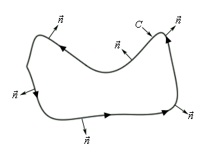
The second form uses the divergence. In this case we also need the outward unit normal to the curve \(C\). If the curve is parameterized by
\[\vec r\left( t \right) = x\left( t \right)\vec i + y\left( t \right)\vec j\]then the outward unit normal is given by,
\[\vec n = \frac{{y'\left( t \right)}}{{\left\| {\vec r'\left( t \right)} \right\|}}\vec i - \frac{{x'\left( t \right)}}{{\left\| {\vec r'\left( t \right)} \right\|}}\vec j\]Here is a sketch illustrating the outward unit normal for some curve \(C\) at various points.
The vector form of Green’s Theorem that uses the divergence is given by,