Section 15.8 : Change of Variables
Back in Calculus I we had the substitution rule that told us that,
\[\int_{{\,a}}^{{\,b}}{{f\left( {g\left( x \right)} \right)\,g'\left( x \right)\,dx}} = \int_{{\,c}}^{{\,d}}{{f\left( u \right)\,du}}\hspace{0.25in}{\mbox{where }}u = g\left( x \right)\]In essence this is taking an integral in terms of \(x\)’s and changing it into terms of \(u\)’s. We want to do something similar for double and triple integrals. In fact we’ve already done this to a certain extent when we converted double integrals to polar coordinates and when we converted triple integrals to cylindrical or spherical coordinates. The main difference is that we didn’t actually go through the details of where the formulas came from. If you recall, in each of those cases we commented that we would justify the formulas for \(dA\) and \(dV\) eventually. Now is the time to do that justification.
While often the reason for changing variables is to get us an integral that we can do with the new variables, another reason for changing variables is to convert the region into a nicer region to work with. When we were converting the polar, cylindrical or spherical coordinates we didn’t worry about this change since it was easy enough to determine the new limits based on the given region. That is not always the case however. So, before we move into changing variables with multiple integrals we first need to see how the region may change with a change of variables.
First, we need a little terminology/notation out of the way. We call the equations that define the change of variables a transformation. Also, we will typically start out with a region, \(R\), in \(xy\)-coordinates and transform it into a region in \(uv\)-coordinates.
- \(R\) is the ellipse \({x^2} + \frac{{{y^2}}}{{36}} = 1\) and the transformation is \(x = \frac{u}{2}\), \(y = 3v\).
- \(R\) is the region bounded by \(y = - x + 4\), \(y = x + 1\), and \(\displaystyle y = \frac{x}{3} - \frac{4}{3}\) and the transformation is \(\displaystyle x = \frac{1}{2}\left( {u + v} \right)\), \(\displaystyle y = \frac{1}{2}\left( {u - v} \right)\).
There really isn’t too much to do with this one other than to plug the transformation into the equation for the ellipse and see what we get.
\[\begin{align*}{\left( {\frac{u}{2}} \right)^2} + \frac{{{{\left( {3v} \right)}^2}}}{{36}} & = 1\\ \frac{{{u^2}}}{4} + \frac{{9{v^2}}}{{36}} & = 1\\ {u^2} + {v^2} & = 4\end{align*}\]So, we started out with an ellipse and after the transformation we had a disk of radius 2.
b \(R\) is the region bounded by \(y = - x + 4\), \(y = x + 1\), and \(\displaystyle y = \frac{x}{3} - \frac{4}{3}\) and the transformation is \(\displaystyle x = \frac{1}{2}\left( {u + v} \right)\), \(\displaystyle y = \frac{1}{2}\left( {u - v} \right)\). Show Solution
As with the first part we’ll need to plug the transformation into the equation, however, in this case we will need to do it three times, once for each equation. Before we do that let’s sketch the graph of the region and see what we’ve got.
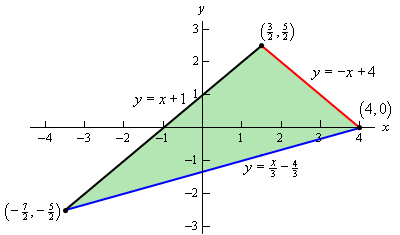
So, we have a triangle. Now, let’s go through the transformation. We will apply the transformation to each edge of the triangle and see where we get.
Let’s do \(y = - x + 4\) first. Plugging in the transformation gives,
\[\begin{align*}\frac{1}{2}\left( {u - v} \right) & = - \frac{1}{2}\left( {u + v} \right) + 4\\ u - v & = - u - v + 8\\ 2u & = 8\\ u & = 4\end{align*}\]The first boundary transforms very nicely into a much simpler equation.
Now let’s take a look at \(y = x + 1\),
\[\begin{align*}\frac{1}{2}\left( {u - v} \right) & = \frac{1}{2}\left( {u + v} \right) + 1\\ u - v & = u + v + 2\\ - 2v & = 2\\ v & = - 1\end{align*}\]Again, a much nicer equation that what we started with.
Finally, let’s transform \(y = \frac{x}{3} - \frac{4}{3}\).
\[\begin{align*}\frac{1}{2}\left( {u - v} \right) & = \frac{1}{3}\left( {\frac{1}{2}\left( {u + v} \right)} \right) - \frac{4}{3}\\ 3u - 3v & = u + v - 8\\ 4v & = 2u + 8\\ v & = \frac{u}{2} + 2\end{align*}\]So, again, we got a somewhat simpler equation, although not quite as nice as the first two.
Let’s take a look at the new region that we get under the transformation.
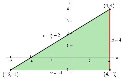
We still get a triangle, but a much nicer one.
Note that we can’t always expect to transform a specific type of region (a triangle for example) into the same kind of region. It is completely possible to have a triangle transform into a region in which each of the edges are curved and in no way resembles a triangle.
Notice that in each of the above examples we took a two dimensional region that would have been somewhat difficult to integrate over and converted it into a region that would be much nicer in integrate over. As we noted at the start of this set of examples, that is often one of the points behind the transformation. In addition to converting the integrand into something simpler it will often also transform the region into one that is much easier to deal with.
Before proceeding with the next topic let’s address another point. On occasion, we will also need to know the range of \(u\) and/or \(v\) for each of the new equations we get from the transformation. We didn’t need that for the two examples above and it is not something that we will often need. However, it can help on occasion in determining the new region.
So, let’s work a quick example to see how we do that.
Okay, we already know what the new region looks like and what the new equations are from the previous example. So, here is a quick review of the transformation of each of the original equations.
\[\begin{align*} & y = - x + 4& \Rightarrow & \hspace{0.25in}u = 4\\ & y = x + 1& \Rightarrow & \hspace{0.25in}v = - 1\\ & y = \frac{x}{3} - \frac{4}{3}& \Rightarrow & \hspace{0.25in}v = \frac{u}{2} + 2\end{align*}\]Here is the new region we get under the transformation.
Note, that, in this case, we could determine the range of \(u\) and \(v\) for each equation from the sketch above. However, in cases where we might actually need the ranges that is usually not an option as we often need the ranges for \(u\) and/or \(v\) to get an accurate sketch of the new region.
So, let’s now actually start working the problem.
Let’s start with the equation \(u = 4\). First, we don’t need a “range” of \(u\)’s here as equation makes it pretty clear we have a single value of \(u\), namely \(u = 4\). So, let’s determine the range of \(v\)’s we should get.
Let’s start with the \(x\) transformation and plug in the known value of \(u\) for this equation. That gives,
\[x = \frac{1}{2}\left( {u + v} \right) = \frac{1}{2}\left( {4 + v} \right)\]Now, we know that the range of \(x\)’s for the original equation, \(y = - x + 4\), are \(\frac{3}{2} \le x \le 4\). We also know from above what \(x\) is in terms of \(v\), so plug that into this range and do a little manipulation as follows,
\[\begin{array}{c}\displaystyle \frac{3}{2} \le x \le 4\\\displaystyle \frac{3}{2} \le \frac{1}{2}\left( {4 + v} \right) \le 4\\ 3 \le 4 + v \le 8\\ - 1 \le v \le 4\end{array}\]So, the range of \(v\)’s for \(u = 4\) must be \( - 1 \le v \le 4\), which nicely matches with what we would expect from the graph of the new region.
Note that we could just as easily used the \(y\) transformation and \(y\) range for the original equation and gotten the same result.
Okay, let’s now move onto \(v = - 1\) and we won’t put in quite as much explanation for this part.
First, we don’t need a range of \(v\) for this because we clearly have just a single value of \(v\). So, to get the range of \(u\) let’s again start with the \(x\) transformation, plug \(v = - 1\) in that and then use the range of \(x\)’s from the original equation, \(y = x + 1\).
Here is that work.
\[\begin{array}{c}\displaystyle - \frac{7}{2} \le x \le \frac{3}{2}\\ \displaystyle - \frac{7}{2} \le \frac{1}{2}\left( {u - 1} \right) \le \frac{3}{2}\\ - 7 \le u - 1 \le 3\\ - 6 \le u \le 4\end{array}\]So, the range of \(u\) for \(v = - 1\) is \( - 6 \le u \le 4\) which, again, matches up with what we see on the graph. Also note that once again, we could have used the \(y\) ranges to do this work.
Finally, let’s find the range of \(u\) and \(v\) for \(v = \frac{u}{2} + 2\). This time let’s use the \(y\) transformation so we can say we used that in one these. So, we’ll start with the range of \(y\)’s for the original equation, \(y = \frac{x}{3} - \frac{4}{3}\), plug in the \(y\) transformation and then plug in for \(v\). Doing this gives,
\[\begin{array}{c} \displaystyle - \frac{5}{2} \le y \le 0\\ \displaystyle - \frac{5}{2} \le \frac{1}{2}\left( {u - \left( {\frac{u}{2} + 2} \right)} \right) \le 0\\ \displaystyle - 5 \le \frac{u}{2} - 2 \le 0\\ \displaystyle - 3 \le \frac{u}{2} \le 2\\ - 6 \le u \le 4\end{array}\]So, again we get the range of \(u\)’s we expect to get from the graph. Once we have those the appropriate range of \(v\) can be found from the equation itself as follows,
\[\begin{array}{c} \displaystyle - 6 \le u \le 4\\ - 3 \le \frac{u}{2} \le 2\\ \displaystyle - 1 \le \frac{u}{2} + 2 \le 4\\ - 1 \le v \le 4\end{array}\]Basically, start with the range of \(u\)’s and “build up” the equation for the side and we get the range of \(v\)’s for this side.
So, we now know how to get ranges of \(u\) and/or \(v\) for new equations under a transformation. However, this is not something that is done terribly often but it is a useful skill to have in case it does arise somewhere.
Now that we’ve seen a couple of examples of transforming regions we need to now talk about how we actually do change of variables in the integral. We will start with double integrals. In order to change variables in a double integral we will need the Jacobian of the transformation. Here is the definition of the Jacobian.
Definition
The Jacobian of the transformation \(x = g\left( {u,v} \right)\), \(y = h\left( {u,v} \right)\) is
\[\frac{{\partial \left( {x,y} \right)}}{{\partial \left( {u,v} \right)}} = \left| {\begin{array}{*{20}{c}}{ \displaystyle \frac{{\partial x}}{{\partial u}}}&{ \displaystyle \frac{{\partial x}}{{\partial v}}}\\{ \displaystyle \frac{{\partial y}}{{\partial u}}}& \displaystyle {\frac{{ \partial y}}{{\partial v}}}\end{array}} \right|\]The Jacobian is defined as a determinant of a 2x2 matrix, if you are unfamiliar with this that is okay. Here is how to compute the determinant.
\[\left| {\begin{array}{*{20}{c}}a&b\\c&d\end{array}} \right| = ad - bc\]Therefore, another formula for the determinant is,
\[\frac{{\partial \left( {x,y} \right)}}{{\partial \left( {u,v} \right)}} = \left| {\begin{array}{*{20}{c}}{ \displaystyle \frac{{\partial x}}{{\partial u}}}&\displaystyle {\frac{{\partial x}}{{\partial v}}}\\{ \displaystyle \frac{{\partial y}}{{\partial u}}}&{ \displaystyle \frac{{\partial y}}{{\partial v}}}\end{array}} \right| = \frac{{\partial x}}{{\partial u}}\frac{{\partial y}}{{\partial v}} - \displaystyle \frac{{\partial x}}{{\partial v}}\frac{{\partial y}}{{\partial u}}\]Now that we have the Jacobian out of the way we can give the formula for change of variables for a double integral.
Change of Variables for a Double Integral
Suppose that we want to integrate \(f\left( {x,y} \right)\) over the region \(R\). Under the transformation \(x = g\left( {u,v} \right)\), \(y = h\left( {u,v} \right)\) the region becomes \(S\) and the integral becomes,
\[\iint\limits_{R}{{f\left( {x,y} \right)\,dA}} = \iint\limits_{S}{{f\left( {g\left( {u,v} \right),h\left( {u,v} \right)} \right)\left| {\frac{{\partial \left( {x,y} \right)}}{{\partial \left( {u,v} \right)}}} \right|\,d\overline{A}}}\]Note that we use \(d\overline{A}\) in the \(u\)/\(v\) integral above to denote that it will be in terms of \(du\) and \(dv\) once we convert to two single integrals rather than the \(dx\) and \(dy\) we are used to using for \(dA\). This is notational only and we generally just use \(dA\) for both and just make sure to remember that the “new” \(dA\) is in terms of \(du\) and \(dv\).
Also note that we are taking the absolute value of the Jacobian.
If we look just at the differentials in the above formula we can also say that
\[dA = \left| {\frac{{\partial \left( {x,y} \right)}}{{\partial \left( {u,v} \right)}}} \right|\,d\overline{A}\]So, what we are doing here is justifying the formula that we used back when we were integrating with respect to polar coordinates. All that we need to do is use the formula above for \(dA\).
The transformation here is the standard conversion formulas,
\[x = r\cos \theta \hspace{0.25in}\hspace{0.25in}y = r\sin \theta \]The Jacobian for this transformation is,
\[\begin{align*}\frac{{\partial \left( {x,y} \right)}}{{\partial \left( {r,\theta } \right)}} & = \left| {\begin{array}{*{20}{c}}{\displaystyle \frac{{\partial x}}{{\partial r}}}&{\displaystyle \frac{{\partial x}}{{\partial \theta }}}\\\displaystyle {\frac{{\partial y}}{{\partial r}}}&\displaystyle {\frac{{\partial y}}{{\partial \theta }}}\end{array}} \right|\\ & = \left| {\begin{array}{*{20}{c}}{\cos \theta }&{ - r\sin \theta }\\{\sin \theta }&{r\cos \theta }\end{array}} \right|\\ & = r{\cos ^2}\theta - \left( { - r{{\sin }^2}\theta } \right)\\ & = r\left( {{{\cos }^2}\theta + {{\sin }^2}\theta } \right)\\ & = r\end{align*}\]We then get,
\[dA = \left| {\frac{{\partial \left( {x,y} \right)}}{{\partial \left( {r,\theta } \right)}}} \right|\,dr\,d\theta = \left| r \right|dr\,d\theta = r\,dr\,d\theta \]So, the formula we used in the section on polar integrals was correct.
Now, let’s do a couple of integrals.
First, let’s sketch the region \(R\) and determine equations for each of the sides.
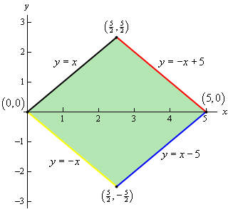
Each of the equations was found by using the fact that we know two points on each line (i.e. the two vertices that form the edge).
While we could do this integral in terms of \(x\) and \(y\) it would involve two integrals and so would be some work.
Let’s use the transformation and see what we get. We’ll do this by plugging the transformation into each of the equations above.
Let’s start the process off with \(y = x\).
\[\begin{align*}2u - 3v & = 2u + 3v\\ 6v & = 0\\ v & = 0\end{align*}\]Transforming \(y = - x\) is similar.
\[\begin{align*}2u - 3v & = - \left( {2u + 3v} \right)\\ 4u & = 0\\ u & = 0\end{align*}\]Next, we’ll transform \(y = - x + 5\).
\[\begin{align*}2u - 3v & = - \left( {2u + 3v} \right) + 5\\ 4u & = 5\\ u & = \frac{5}{4}\end{align*}\]Finally, let’s transform \(y = x - 5\).
\[\begin{align*}2u - 3v & = 2u + 3v - 5\\ - 6v & = - 5\\ v & = \frac{5}{6}\end{align*}\]The region \(S\) is then a rectangle whose sides are given by \(u = 0\), \(v = 0\), \(u = \frac{5}{4}\) and \(v = \frac{5}{6}\) and so the ranges of \(u\) and \(v\) are,
\[0 \le u \le \frac{5}{4}\hspace{0.25in}\hspace{0.25in}0 \le v \le \frac{5}{6}\]Next, we need the Jacobian.
\[\frac{{\partial \left( {x,y} \right)}}{{\partial \left( {u,v} \right)}} = \left| {\begin{array}{*{20}{c}}2&3\\2&{ - 3}\end{array}} \right| = - 6 - 6 = - 12\]The integral is then,
\[\begin{align*}\iint\limits_{R}{{x + y\,dA}} & = \int_{{\,0}}^{{\,\frac{5}{6}}}{{\int_{{\,0}}^{{\,\frac{5}{4}}}{{\left( {\left( {2u + 3v} \right) + \left( {2u - 3v} \right)} \right)\left| { - 12} \right|}}\,d\overline{A}}}\\ & = \int_{{\,0}}^{{\,\frac{5}{6}}}{{\int_{{\,0}}^{{\,\frac{5}{4}}}{{48u}}\,d\overline{A}}}\\ & = \int_{{\,0}}^{{\,\frac{5}{6}}}{{\left. {24{u^2}} \right|_0^{\frac{5}{4}}\,dv}}\\ & = \int_{{\,0}}^{{\,\frac{5}{6}}}{{\frac{{75}}{2}\,dv}}\\ & = \left. {\frac{{75}}{2}v} \right|_0^{\frac{5}{6}}\\ & = \frac{{125}}{4}\end{align*}\]Before we proceed with this problem. Let’s do a quick graph of the boundary of the region \(R\). We claimed that it is an ellipse, but is clearly not in “standard” form. Here is the boundary of \(R\).
So, it is an ellipse, just one that is at an angle rather than symmetric about the \(x\) and \(y\)-axis as we are used to dealing with.
Also, note that we used “\( \le 2\)” when “defining” \(R\) to make it clear that we are using both the actual ellipse itself as well as the interior of the ellipse for \(R\).
Okay, let’s proceed with the problem.
The first thing to do is to plug the transformation into the equation for the ellipse to see what the region transforms into.
\[\begin{align*}2 & = {x^2} - xy + {y^2}\\ & = {\left( {\sqrt 2 \,u - \sqrt {\frac{2}{3}} \,v} \right)^2} - \left( {\sqrt 2 \,u - \sqrt {\frac{2}{3}} \,v} \right)\left( {\sqrt 2 \,u + \sqrt {\frac{2}{3}} \,v} \right) + {\left( {\sqrt 2 \,u + \sqrt {\frac{2}{3}} \,v} \right)^2}\\ & = 2{u^2} - \frac{4}{{\sqrt 3 }}uv + \frac{2}{3}{v^2} - \left( {2{u^2} - \frac{2}{3}{v^2}} \right) + 2{u^2} + \frac{4}{{\sqrt 3 }}uv + \frac{2}{3}{v^2}\\ & = 2{u^2} + 2{v^2}\end{align*}\]Or, upon dividing by 2 we see that the equation describing \(R\) transforms into
\[{u^2} + {v^2} = 1\]or the unit circle. Again, this will be much easier to integrate over than the original region.
Note as well that we’ve shown that the function that we’re integrating is
\[{x^2} - xy + {y^2} = 2\left( {{u^2} + {v^2}} \right)\]in terms of \(u\) and \(v\) so we won’t have to redo that work when the time to do the integral comes around.
Finally, we need to find the Jacobian.
\[\frac{{\partial \left( {x,y} \right)}}{{\partial \left( {u,v} \right)}} = \left| {\begin{array}{*{20}{c}}{\sqrt 2 }&{ - \sqrt {\frac{2}{3}} }\\{\sqrt 2 }&{\sqrt {\frac{2}{3}} }\end{array}} \right| = \frac{2}{{\sqrt 3 }} + \frac{2}{{\sqrt 3 }} = \frac{4}{{\sqrt 3 }}\]The integral is then,
\[\iint\limits_{R}{{{x^2} - xy + {y^2}\,dA}} = \iint\limits_{S}{{2\left( {{u^2} + {v^2}} \right)\left| {\frac{4}{{\sqrt 3 }}} \right|\,du\,dv}}\]Before proceeding a word of caution is in order. Do not make the mistake of substituting \({x^2} - xy + {y^2} = 2\) or \({u^2} + {v^2} = 1\) in for the integrand. These equations are only valid on the boundary of the region and we are looking at all the points interior to the boundary as well and for those points neither of these equations will be true!
At this point we’ll note that this integral will be much easier in terms of polar coordinates and so to finish the integral out will convert to polar coordinates.
\[\begin{align*}\iint\limits_{R}{{{x^2} - xy + {y^2}\,dA}} & = \iint\limits_{S}{{2\left( {{u^2} + {v^2}} \right)\left| {\frac{4}{{\sqrt 3 }}} \right|\,du\,dv}}\\ & = \frac{8}{{\sqrt 3 }}\int_{{\,0}}^{{\,2\pi }}{{\int_{{\,0}}^{{\,1}}{{\left( {{r^2}} \right)r\,dr}}\,d\theta }}\\ & = \frac{8}{{\sqrt 3 }}\int_{0}^{{2\pi }}{{\left. {\frac{1}{4}{r^4}} \right|_0^1\,d\theta }}\\ & = \frac{8}{{\sqrt 3 }}\int_{0}^{{2\pi }}{{\frac{1}{4}\,d\theta }}\\ & = \frac{{4\pi }}{{\sqrt 3 }}\end{align*}\]Let’s now briefly look at triple integrals. In this case we will again start with a region \(R\) and use the transformation \(x = g\left( {u,v,w} \right)\), \(y = h\left( {u,v,w} \right)\), and \(z = k\left( {u,v,w} \right)\) to transform the region into the new region \(S\). To do the integral we will need a Jacobian, just as we did with double integrals. Here is the definition of the Jacobian for this kind of transformation.
\[\frac{{\partial \left( {x,y,z} \right)}}{{\partial \left( {u,v,w} \right)}} = \left| {\begin{array}{*{20}{c}}{ \displaystyle \frac{{\partial x}}{{\partial u}}}& \displaystyle {\frac{{\partial x}}{{\partial v}}}& \displaystyle {\frac{{\partial x}}{{\partial w}}}\\ \displaystyle {\frac{{\partial y}}{{\partial u}}}& \displaystyle {\frac{{\partial y}}{{\partial v}}}& \displaystyle {\frac{{\partial y}}{{\partial w}}}\\ \displaystyle{\frac{{\partial z}}{{\partial u}}}& \displaystyle {\frac{{\partial z}}{{\partial v}}}& \displaystyle {\frac{{\partial z}}{{\partial w}}}\end{array}} \right|\]In this case the Jacobian is defined in terms of the determinant of a 3x3 matrix. We saw how to evaluate these when we looked at cross products back in Calculus II. If you need a refresher on how to compute them you should go back and review that section.
The integral under this transformation is,
\[\iiint\limits_{R}{{f\left( {x,y,z} \right)\,dV}} = \iiint\limits_{S}{{f\left( {g\left( {u,v,w} \right),h\left( {u,v,w} \right),k\left( {u,v,w} \right)} \right)\left| {\frac{{\partial \left( {x,y,z} \right)}}{{\partial \left( {u,v,w} \right)}}} \right|\,d\overline{V}}}\]As with double integrals we used \(d\overline{V}\) in the \(u\)/\(v\)/\(w\) integral above to remind ourselves that we will need to use \(du\), \(dv\) and \(dw\) when converting to single integrals. Again, this is just notation and is usually written as just \(dV\).
We can look at just the differentials and note that we must have
\[dV = \left| {\frac{{\partial \left( {x,y,z} \right)}}{{\partial \left( {u,v,w} \right)}}} \right|\,d\overline{V}\]We’re not going to do any integrals here, but let’s verify the formula for \(dV\) for spherical coordinates.
Here the transformation is just the standard conversion formulas.
\[x = \rho \sin \varphi \cos \theta \hspace{0.25in}y = \rho \sin \varphi \sin \theta \hspace{0.25in}z = \rho \cos \varphi \]The Jacobian is,
\[\begin{align*}\frac{{\partial \left( {x,y,z} \right)}}{{\partial \left( {\rho ,\theta ,\varphi } \right)}} & = \left| {\begin{array}{*{20}{c}}{\sin \varphi \cos \theta }&{ - \rho \sin \varphi \sin \theta }&{\rho \cos \varphi \cos \theta }\\{\sin \varphi \sin \theta }&{\rho \sin \varphi \cos \theta }&{\rho \cos \varphi \sin \theta }\\{\cos \varphi }&0&{ - \rho \sin \varphi }\end{array}} \right|\\ & = - \rho ^2\sin ^3\varphi \cos^2\theta - \rho^2 \sin \varphi \cos ^2\varphi \sin^2\theta + 0\\ & \hspace{0.75in} - \rho^2 \sin^3 \varphi \sin^2 \theta - 0 - \rho^2 \sin \varphi \cos^2\varphi {\cos ^2}\theta \\ & = - {\rho ^2}\sin^3\varphi \left( {{{\cos }^2}\theta + {{\sin }^2}\theta } \right) - \rho^2 \sin \varphi \cos^2 \varphi \left( {{{\sin }^2}\theta + {{\cos }^2}\theta } \right)\\ & = - {\rho ^2}{\sin ^3}\varphi - \rho ^2 \sin \varphi \cos^2 \varphi \\ & = - {\rho ^2}\sin \varphi \left( {{{\sin }^2}\varphi + {{\cos }^2}\varphi } \right)\\ & = - {\rho ^2}\sin \varphi \end{align*}\]Finally, \(dV\) becomes,
\[dV = \left| { - {\rho ^2}\sin \varphi } \right|\,d\rho \,d\theta \,d\varphi = {\rho ^2}\sin \varphi \,d\rho \,d\theta \,d\varphi \]Recall that we restricted \(\varphi \) to the range \(0 \le \varphi \le \pi \) for spherical coordinates and so we know that \(\sin \varphi \ge 0\) and so we don’t need the absolute value bars on the sine.
We will leave it to you to check the formula for \(dV\) for cylindrical coordinates if you’d like to. It is a much easier formula to check.