Section 14.4 : Absolute Extrema
In this section we are going to extend the work from the previous section. In the previous section we were asked to find and classify all critical points as relative minimums, relative maximums and/or saddle points. In this section we want to optimize a function, that is identify the absolute minimum and/or the absolute maximum of the function, on a given region in \({\mathbb{R}^2}\). Note that when we say we are going to be working on a region in \({\mathbb{R}^2}\) we mean that we’re going to be looking at some region in the xy-plane.
In order to optimize a function in a region we are going to need to get a couple of definitions out of the way and a fact. Let’s first get the definitions out of the way.
Definitions
- A region in \({\mathbb{R}^2}\) is called closed if it includes its boundary. A region is called open if it doesn’t include any of its boundary points.
- A region in \({\mathbb{R}^2}\) is called bounded if it can be completely contained in a disk. In other words, a region will be bounded if it is finite.
Let’s think a little more about the definition of closed. We said a region is closed if it includes its boundary. Just what does this mean? Let’s think of a rectangle. Below are two definitions of a rectangle, one is closed and the other is open.
\[\begin{array}{*{20}{c}}\begin{aligned}{\mbox{Open}} \,\,\,\,\,\, \\ - 5 < x < 3\\ \,\,\,1 < y < 6\end{aligned}&\begin{aligned}{\mbox{Closed}}\,\,\,\,\,\\ \hspace{0.25in} - 5 \le x \le 3\\ \,\,\,\hspace{0.25in}\,\,\,1 \le y \le 6\end{aligned}\end{array}\]In this first case we don’t allow the ranges to include the endpoints (i.e. we aren’t including the edges of the rectangle) and so we aren’t allowing the region to include any points on the edge of the rectangle. In other words, we aren’t allowing the region to include its boundary and so it’s open.
In the second case we are allowing the region to contain points on the edges and so will contain its entire boundary and hence will be closed.
This is an important idea because of the following fact.
Extreme Value Theorem
If \(f\left( {x,y} \right)\) is continuous in some closed, bounded set \(D\) in \({\mathbb{R}^2}\) then there are points in \(D\), \(\left( {{x_1},{y_1}} \right)\) and \(\left( {{x_2},{y_2}} \right)\) so that \(f\left( {{x_1},{y_1}} \right)\) is the absolute maximum and \(f\left( {{x_2},{y_2}} \right)\) is the absolute minimum of the function in \(D\).
Note that this theorem does NOT tell us where the absolute minimum or absolute maximum will occur. It only tells us that they will exist. Note as well that the absolute minimum and/or absolute maximum may occur in the interior of the region or it may occur on the boundary of the region.
The basic process for finding absolute maximums is pretty much identical to the process that we used in Calculus I when we looked at finding absolute extrema of functions of single variables. There will however, be some procedural changes to account for the fact that we now are dealing with functions of two variables. Here is the process.
Finding Absolute Extrema
- Find all the critical points of the function that lie in the region \(D\) and determine the function value at each of these points.
- Find all extrema of the function on the boundary. This usually involves the Calculus I approach for this work.
- The largest and smallest values found in the first two steps are the absolute minimum and the absolute maximum of the function.
The main difference between this process and the process that we used in Calculus I is that the “boundary” in Calculus I was just two points and so there really wasn’t a lot to do in the second step. For these problems the majority of the work is often in the second step as we will often end up doing a Calculus I absolute extrema problem one or more times.
Let’s take a look at an example or two.
Let’s first get a quick picture of the rectangle for reference purposes.
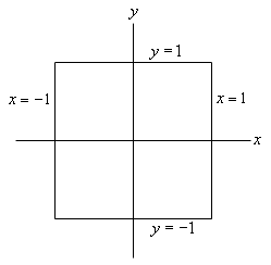
The boundary of this rectangle is given by the following conditions.
\[\begin{align*}&{\mbox{right side :}}\hspace{0.25in}x = 1,\,\, - 1 \le y \le 1\\ & {\mbox{left side :}}\hspace{0.25in}x = - 1,\,\, - 1 \le y \le 1\\ & {\mbox{upper side :}}\hspace{0.25in}y = 1,\,\, - 1 \le x \le 1\\ & {\mbox{lower side :}}\hspace{0.25in}y = - 1,\,\, - 1 \le x \le 1\end{align*}\]These will be important in the second step of our process.
We’ll start this off by finding all the critical points that lie inside the given rectangle. To do this we’ll need the two first order derivatives.
\[{f_x} = 2x - 4xy\hspace{0.5in}{f_y} = 8y - 2{x^2}\]Note that since we aren’t going to be classifying the critical points we don’t need the second order derivatives. To find the critical points we will need to solve the system,
\[\begin{align*}2x - 4xy & = 0\\ 8y - 2{x^2} & = 0\end{align*}\]We can solve the second equation for \(y\) to get,
\[y = \frac{{{x^2}}}{4}\]Plugging this into the first equation gives us,
\[2x - 4x\left( {\frac{{{x^2}}}{4}} \right) = 2x - {x^3} = x\left( {2 - {x^2}} \right) = 0\]This tells us that we must have \(x = 0\) or \(x = \pm \sqrt 2 = \pm 1.414...\). Now, recall that we only want critical points in the region that we’re given. That means that we only want critical points for which \( - 1 \le x \le 1\). The only value of \(x\) that will satisfy this is the first one so we can ignore the last two for this problem. Note however that a simple change to the boundary would include these two so don’t forget to always check if the critical points are in the region (or on the boundary since that can also happen).
Plugging \(x = 0\) into the equation for \(y\) gives us,
\[y = \frac{{{0^2}}}{4} = 0\]The single critical point, in the region (and again, that’s important), is \(\left( {0,0} \right)\). We now need to get the value of the function at the critical point.
\[f\left( {0,0} \right) = 4\]Eventually we will compare this to values of the function found in the next step and take the largest and smallest as the absolute extrema of the function in the rectangle.
Now we have reached the long part of this problem. We need to find the absolute extrema of the function along the boundary of the rectangle. What this means is that we’re going to need to look at what the function is doing along each of the sides of the rectangle listed above.
Let’s first take a look at the right side. As noted above the right side is defined by
\[x = 1,\,\, - 1 \le y \le 1\]Notice that along the right side we know that \(x = 1\). Let’s take advantage of this by defining a new function as follows,
\[g\left( y \right) = f\left( {1,y} \right) = {1^2} + 4{y^2} - 2\left( {{1^2}} \right)y + 4 = 5 + 4{y^2} - 2y\]Now, finding the absolute extrema of \(f\left( {x,y} \right)\) along the right side will be equivalent to finding the absolute extrema of \(g\left( y \right)\) in the range \( - 1 \le y \le 1\). Hopefully you recall how to do this from Calculus I. We find the critical points of \(g\left( y \right)\) in the range \( - 1 \le y \le 1\) and then evaluate \(g\left( y \right)\) at the critical points and the end points of the range of \(y\)’s.
Let’s do that for this problem.
\[g'\left( y \right) = 8y - 2\hspace{0.5in} \Rightarrow \hspace{0.25in}\,\,\,\,\,y = \frac{1}{4}\]This is in the range and so we will need the following function evaluations.
\[g\left( { - 1} \right) = 11\hspace{0.5in}g\left( 1 \right) = 7\hspace{0.5in}g\left( {\frac{1}{4}} \right) = \frac{{19}}{4} = 4.75\]Notice that, using the definition of \(g\left( y \right)\) these are also function values for \(f\left( {x,y} \right)\).
\[\begin{align*}g\left( { - 1} \right) & = f\left( {1, - 1} \right) = 11\hspace{0.5in}\\ g\left( 1 \right) & = f\left( {1,1} \right) = 7\\ g\left( {\frac{1}{4}} \right) & = f\left( {1,\frac{1}{4}} \right) = \frac{{19}}{4} = 4.75\end{align*}\]We can now do the left side of the rectangle which is defined by,
\[x = - 1,\,\, - 1 \le y \le 1\]Again, we’ll define a new function as follows,
\[g\left( y \right) = f\left( { - 1,y} \right) = {\left( { - 1} \right)^2} + 4{y^2} - 2{\left( { - 1} \right)^2}y + 4 = 5 + 4{y^2} - 2y\]Notice however that, for this boundary, this is the same function as we looked at for the right side. This will not always happen, but since it has let’s take advantage of the fact that we’ve already done the work for this function. We know that the critical point is \(y = \frac{1}{4}\) and we know that the function value at the critical point and the end points are,
\[g\left( { - 1} \right) = 11\hspace{0.5in}g\left( 1 \right) = 7\hspace{0.5in}g\left( {\frac{1}{4}} \right) = \frac{{19}}{4} = 4.75\]The only real difference here is that these will correspond to values of \(f\left( {x,y} \right)\) at different points than for the right side. In this case these will correspond to the following function values for \(f\left( {x,y} \right)\).
\[\begin{align*}g\left( { - 1} \right) & = f\left( { - 1, - 1} \right) = 11\hspace{0.5in}\\ g\left( 1 \right) & = f\left( { - 1,1} \right) = 7\\ g\left( {\frac{1}{4}} \right) & = f\left( { - 1,\frac{1}{4}} \right) = \frac{{19}}{4} = 4.75\end{align*}\]We can now look at the upper side defined by,
\[y = 1,\,\, - 1 \le x \le 1\]We’ll again define a new function except this time it will be a function of \(x\).
\[h\left( x \right) = f\left( {x,1} \right) = {x^2} + 4\left( {{1^2}} \right) - 2{x^2}\left( 1 \right) + 4 = 8 - {x^2}\]We need to find the absolute extrema of \(h\left( x \right)\) on the range \( - 1 \le x \le 1\). First find the critical point(s).
\[h'\left( x \right) = - 2x\hspace{0.5in} \Rightarrow \hspace{0.5in}x = 0\]The value of this function at the critical point and the end points is,
\[h\left( { - 1} \right) = 7\hspace{0.5in}h\left( 1 \right) = 7\hspace{0.5in}h\left( 0 \right) = 8\]and these in turn correspond to the following function values for \(f\left( {x,y} \right)\)
\[\begin{align*}h\left( { - 1} \right) & = f\left( { - 1,1} \right) = 7\\ h\left( 1 \right) & = f\left( {1,1} \right) = 7\\ h\left( 0 \right) & = f\left( {0,1} \right) = 8\end{align*}\]Note that there are several “repeats” here. The first two function values have already been computed when we looked at the right and left side. This will often happen.
Finally, we need to take care of the lower side. This side is defined by,
\[y = - 1,\,\, - 1 \le x \le 1\]The new function we’ll define in this case is,
\[h\left( x \right) = f\left( {x, - 1} \right) = {x^2} + 4{\left( { - 1} \right)^2} - 2{x^2}\left( { - 1} \right) + 4 = 8 + 3{x^2}\]The critical point for this function is,
\[h'\left( x \right) = 6x\hspace{0.5in} \Rightarrow \hspace{0.5in}x = 0\]The function values at the critical point and the endpoint are,
\[h\left( { - 1} \right) = 11\hspace{0.5in}h\left( 1 \right) = 11\hspace{0.5in}h\left( 0 \right) = 8\]and the corresponding values for \(f\left( {x,y} \right)\) are,
\[\begin{align*}h\left( { - 1} \right) & = f\left( { - 1, - 1} \right) = 11\\ h\left( 1 \right) & = f\left( {1, - 1} \right) = 11\\ h\left( 0 \right) & = f\left( {0, - 1} \right) = 8\end{align*}\]The final step to this (long…) process is to collect up all the function values for \(f\left( {x,y} \right)\) that we’ve computed in this problem. Here they are,
\[\begin{align*}f\left( {0,0} \right) & = 4\hspace{0.5in} & f\left( {1, - 1} \right) & = 11\hspace{0.5in} & f\left( {1,1} \right) & = 7\\ f\left( {1,\frac{1}{4}} \right) & = 4.75\hspace{0.5in} & f\left( { - 1,1} \right) & = 7\hspace{0.5in} & f\left( { - 1, - 1} \right) & = 11\\ f\left( { - 1,\frac{1}{4}} \right) & = 4.75\hspace{0.25in} & f\left( {0,1} \right) & = 8\hspace{0.5in} & f\left( {0, - 1} \right) & = 8\end{align*}\]The absolute minimum is at \(\left( {0,0} \right)\) since gives the smallest function value and the absolute maximum occurs at \(\left( {1, - 1} \right)\) and \(\left( { - 1, - 1} \right)\) since these two points give the largest function value.
Here is a sketch of the function on the rectangle for reference purposes.
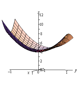
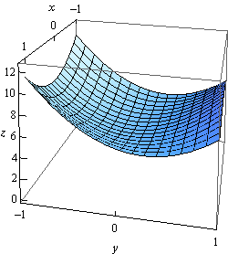
As this example has shown these can be very long problems on occasion. Let’s take a look at an easier, well shorter anyway, problem with a different kind of boundary.
First note that a disk of radius 4 is given by the inequality in the problem statement. The “less than” inequality is included to get the interior of the disk and the equal sign is included to get the boundary. Of course, this also means that the boundary of the disk is a circle of radius 4.
Let’s first find the critical points of the function that lies inside the disk. This will require the following two first order partial derivatives.
\[{f_x} = 4x\hspace{0.5in}{f_y} = - 2y + 6\]To find the critical points we’ll need to solve the following system.
\[\begin{align*}4x & = 0\\- 2y + 6 & = 0\end{align*}\]This is actually a fairly simple system to solve however. The first equation tells us that \(x = 0\) and the second tells us that \(y = 3\). So, the only critical point for this function is \(\left( {0,3} \right)\) and this is inside the disk of radius 4. The function value at this critical point is,
\[f\left( {0,3} \right) = 9\]Now we need to look at the boundary. This one will be somewhat different from the previous example. In this case we don’t have fixed values of \(x\) and \(y\) on the boundary. Instead we have,
\[{x^2} + {y^2} = 16\]We can solve this for \({x^2}\) and plug this into the \({x^2}\) in \(f\left( {x,y} \right)\) to get a function of \(y\) as follows.
\[{x^2} = 16 - {y^2}\] \[g\left( y \right) = 2\left( {16 - {y^2}} \right) - {y^2} + 6y = 32 - 3{y^2} + 6y\]We will need to find the absolute extrema of this function on the range \( - 4 \le y \le 4\) (this is the range of \(y\)’s for the disk….). We’ll first need the critical points of this function.
\[g'\left( y \right) = - 6y + 6\hspace{0.25in} \Rightarrow \hspace{0.25in}\,\,\,y = 1\]The value of this function at the critical point and the endpoints are,
\[g\left( { - 4} \right) = - 40\hspace{0.5in}g\left( 4 \right) = 8\hspace{0.25in}\,\,\,\,\,\,g\left( 1 \right) = 35\]Unlike the first example we will still need to find the values of \(x\) that correspond to these. We can do this by plugging the value of \(y\) into our equation for the circle and solving for \(x\).
\[\begin{align*} & y = - 4 : & {x^2} & = 16 - 16 = 0\hspace{0.25in} \Rightarrow \hspace{0.25in}x = 0\\ & y = 4 : &{x^2} & = 16 - 16 = 0\hspace{0.25in} \Rightarrow \hspace{0.25in}x = 0\\ & y = 1 : & {x^2} & = 16 - 1 = 15\hspace{0.25in} \Rightarrow \hspace{0.25in}x = \pm \sqrt {15} = \pm 3.87\end{align*}\]The function values for \(g\left( y \right)\) then correspond to the following function values for \(f\left( {x,y} \right)\).
\[\begin{align*}g\left( { - 4} \right) & = - 40 & \Rightarrow & \hspace{0.25in}f\left( {0, - 4} \right) = - 40\\ g\left( 4 \right) & = 8 & \Rightarrow & \hspace{0.25in}f\left( {0,4} \right) = 8\\ g\left( 1 \right) & = 35 & \Rightarrow & \hspace{0.25in}f\left( { - \sqrt {15} ,1} \right) = 35\,\,\,\,{\mbox{and}}\,\,\,\,\,f\left( {\sqrt {15} ,1} \right) = 35\end{align*}\]Note that the third one actually corresponded to two different values for \(f\left( {x,y} \right)\) since that \(y\) also produced two different values of \(x\).
So, comparing these values to the value of the function at the critical point of \(f\left( {x,y} \right)\) that we found earlier we can see that the absolute minimum occurs at \(\left( {0, - 4} \right)\) while the absolute maximum occurs twice at \(\left( { - \sqrt {15} ,1} \right)\) and \(\left( {\sqrt {15} ,1} \right)\).
Here is a sketch of the region for reference purposes.
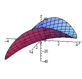
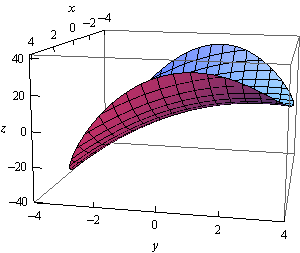
In both of these examples one of the absolute extrema actually occurred at more than one place. Sometimes this will happen and sometimes it won’t so don’t read too much into the fact that it happened in both examples given here.
Also note that, as we’ve seen, absolute extrema will often occur on the boundaries of these regions, although they don’t have to occur at the boundaries. Had we given much more complicated examples with multiple critical points we would have seen examples where the absolute extrema occurred interior to the region and not on the boundary.