Let’s first divide both sides by \({x^2}\) to rewrite the differential equation as follows,

\[\frac{y}{x}\,y' = - 4 - \frac{{{y^2}}}{{{x^2}}} = - 4 - {\left( {\frac{y}{x}} \right)^2}\]

Now, this is not in the officially proper form as we have listed above, but we can see that everywhere the variables are listed they show up as the ratio, \({y}/{x}\;\) and so this is really as far as we need to go. So, let’s plug the substitution into this form of the differential equation to get,

\[v\left( {v + xv'} \right) = - 4 - {v^2}\]

Next, rewrite the differential equation to get everything separated out.

\[\begin{align*}v\,x\,v' & = - 4 - 2{v^2}\\ x\,v' & = - \frac{{4 + 2{v^2}}}{v}\\ \frac{v}{{4 + 2{v^2}}}dv & = - \frac{1}{x}dx\end{align*}\]

Integrating both sides gives,

\[\frac{1}{4}\ln \left( {4 + 2{v^2}} \right) = - \ln \left( x \right) + c\]

We need to do a little rewriting using basic logarithm properties in order to be able to easily solve this for \(v\).

\[\ln {\left( {4 + 2{v^2}} \right)^{\frac{1}{4}}} = \ln {\left( x \right)^{ - 1}} + c\]

Now exponentiate both sides and do a little rewriting

\[{\left( {4 + 2{v^2}} \right)^{\frac{1}{4}}} = {{\bf{e}}^{\,\ln {{\left( x \right)}^{ - 1}} + c}} = {{\bf{e}}^c}{{\bf{e}}^{\,\ln {{\left( x \right)}^{ - 1}}}} = \frac{c}{x}\]

Note that because \(c\) is an unknown constant then so is \({{\bf{e}}^{\,c}}\) and so we may as well just call this \(c\) as we did above.

Finally, let’s solve for \(v\) and then plug the substitution back in and we’ll play a little fast and loose with constants again.

\[\begin{align*}4 + 2{v^2} & = \frac{{{c^4}}}{{{x^4}}} = \frac{c}{{{x^4}}}\\ {v^2} & = \frac{1}{2}\left( {\frac{c}{{{x^4}}} - 4} \right)\\ \frac{{{y^2}}}{{{x^2}}} & = \frac{1}{2}\left( {\frac{{c - 4{x^4}}}{{{x^4}}}} \right)\\ {y^2} & = \frac{1}{2}{x^2}\left( {\frac{{c - 4{x^4}}}{{{x^4}}}} \right) = \frac{{c - 4{x^4}}}{{2{x^2}}}\end{align*}\]

At this point it would probably be best to go ahead and apply the initial condition. Doing that gives,

\[49 = \frac{{c - 4\left( {16} \right)}}{{2\left( 4 \right)}}\hspace{0.25in} \Rightarrow \hspace{0.25in}c = 456\]

Note that we could have also converted the original initial condition into one in terms of \(v\) and then applied it upon solving the separable differential equation. In this case however, it was probably a little easier to do it in terms of \(y\) given all the logarithms in the solution to the separable differential equation.

Finally, plug in \(c\) and solve for \(y\) to get,

\[{y^2} = \frac{{228 - 2{x^4}}}{{{x^2}}}\hspace{0.25in} \Rightarrow \hspace{0.25in}y\left( x \right) = \pm \sqrt {\frac{{228 - 2{x^4}}}{{{x^2}}}} \]

The initial condition tells us that the “–” must be the correct sign and so the actual solution is,

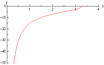
\[y\left( x \right) = - \sqrt {\frac{{228 - 2{x^4}}}{{{x^2}}}} \]

For the interval of validity we can see that we need to avoid \(x = 0\) and because we can’t allow negative numbers under the square root we also need to require that,

\[\begin{align*}228 - 2{x^4} & \ge 0\\ {x^4} & \le 114\hspace{0.25in} \Rightarrow \hspace{0.25in} - 3.2676 \le x \le 3.2676\end{align*}\]

So, we have two possible intervals of validity,

\[ - 3.2676 \le x < 0\hspace{0.25in}0 < x \le 3.2676\]

and the initial condition tells us that it must be \(0 < x \le 3.2676\).

The graph of the solution is,

On the surface this differential equation looks like it won’t be homogeneous. However, with a quick logarithm property we can rewrite this as,

\[y' = \frac{y}{x}\ln \left( {\frac{x}{y}} \right)\]

In this form the differential equation is clearly homogeneous. Applying the substitution and separating gives,

\[\begin{align*}v + xv' & = v\ln \left( {\frac{1}{v}} \right)\\ xv' & = v\left( {\ln \left( {\frac{1}{v}} \right) - 1} \right)\\ \frac{{dv}}{{v\left( {\ln \left( {\frac{1}{v}} \right) - 1} \right)}} & = \frac{{dx}}{x}\end{align*}\]

Integrate both sides and do a little rewrite to get,

\[\begin{align*} - \ln \left( {\ln \left( {\frac{1}{v}} \right) - 1} \right) & = \ln x + c\\ \ln \left( {\ln \left( {\frac{1}{v}} \right) - 1} \right) & = c - \ln x\end{align*}\]

You were able to do the integral on the left right? It used the substitution \(u = \ln \left( {\frac{1}{v}} \right) - 1\).

Now, solve for \(v\) and note that we’ll need to exponentiate both sides a couple of times and play fast and loose with constants again.

\[\begin{align*}\ln \left( {\frac{1}{v}} \right) - 1 = {{\bf{e}}^{\,\ln {{\left( x \right)}^{ - 1}} + c}} & = {{\bf{e}}^c}{{\bf{e}}^{\,\ln {{\left( x \right)}^{ - 1}}}} = \frac{c}{x}\\ \ln \left( {\frac{1}{v}} \right) & = \frac{c}{x} + 1\\ \frac{1}{v} & = {{\bf{e}}^{\,\frac{c}{x} + 1}}\hspace{0.25in} \Rightarrow \hspace{0.25in}v = {{\bf{e}}^{ - \,\,\frac{c}{x}\, - \,1}}\end{align*}\]

Plugging the substitution back in and solving for \(y\) gives,

\[\frac{y}{x} = {{\bf{e}}^{ - \,\,\frac{c}{x}\, - \,1}}\hspace{0.25in} \Rightarrow \hspace{0.25in}y\left( x \right) = x{{\bf{e}}^{ - \,\,\frac{c}{x}\, - \,1}}\]

Applying the initial condition and solving for \(c\) gives,

\[4 = {{\bf{e}}^{ - \,c\, - \,1}}\hspace{0.25in} \Rightarrow \hspace{0.25in}c = - \left( {1 + \ln 4} \right)\]

The solution is then,

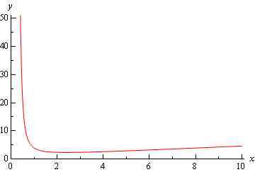
\[y\left( x \right) = x{{\bf{e}}^{\,\frac{{1 + \ln 4}}{x}\, - \,1}}\]

We clearly need to avoid \(x = 0\) to avoid division by zero and so with the initial condition we can see that the interval of validity is \(x > 0\).

The graph of the solution is,

In this case we’ll use the substitution.

\[v = 4x - y\hspace{0.25in}v' = 4 - y'\]

Note that we didn’t include the “+1” in our substitution. Usually only the \(ax + by\) part gets included in the substitution. There are times where including the extra constant may change the difficulty of the solution process, either easier or harder, however in this case it doesn’t really make much difference so we won’t include it in our substitution.

So, plugging this into the differential equation gives,

\[\begin{align*}4 - v' - {\left( {v + 1} \right)^2} & = 0\\ v' & = 4 - {\left( {v + 1} \right)^2}\\ \frac{{dv}}{{{{\left( {v + 1} \right)}^2} - 4}} & = - dx\end{align*}\]

As we’ve shown above we definitely have a separable differential equation. Also note that to help with the solution process we left a minus sign on the right side. We’ll need to integrate both sides and in order to do the integral on the left we’ll need to use partial fractions. We’ll leave it to you to fill in the missing details and given that we’ll be doing quite a bit of partial fraction work in a few chapters you should really make sure that you can do the missing details.

\[\begin{align*}\int{{\frac{{dv}}{{{v^2} + 2v - 3}}}} = \int{{\frac{{dv}}{{\left( {v + 3} \right)\left( {v - 1} \right)}}}} & = \int{{ - dx}}\\ \frac{1}{4}\int{{\frac{1}{{v - 1}} - \frac{1}{{v + 3}}dv}} & = \int{{ - dx}}\\ \frac{1}{4}\left( {\ln \left( {v - 1} \right) - \ln \left( {v + 3} \right)} \right) & = - x + c\\ \ln \left( {\frac{{v - 1}}{{v + 3}}} \right) & = c - 4x\end{align*}\]

Note that we played a little fast and loose with constants above. The next step is fairly messy but needs to be done and that is to solve for \(v\) and note that we’ll be playing fast and loose with constants again where we can get away with it and we’ll be skipping a few steps that you shouldn’t have any problem verifying.

\[\begin{align*}\frac{{v - 1}}{{v + 3}} = {{\bf{e}}^{c - 4x\,}} & = c\,{{\bf{e}}^{ - 4x\,}}\\ v - 1 & = c\,{{\bf{e}}^{ - 4x\,}}\left( {v + 3} \right)\\ v\left( {1 - c\,{{\bf{e}}^{ - 4x\,}}} \right) & = 1 + 3c\,{{\bf{e}}^{ - 4x\,}}\end{align*}\]

At this stage we should back away a bit and note that we can’t play fast and loose with constants anymore. We were able to do that in first step because the \(c\) appeared only once in the equation. At this point however, the \(c\) appears twice and so we’ve got to keep them around. If we “absorbed” the 3 into the \(c\) on the right the “new” \(c\) would be different from the \(c\) on the left because the \(c\) on the left didn’t have the 3 as well.

So, let’s solve for \(v\) and then go ahead and go back into terms of \(y\).

\[\begin{align*}v & = \frac{{1 + 3c\,{{\bf{e}}^{ - 4x\,}}}}{{1 - c\,{{\bf{e}}^{ - 4x\,}}}}\\ 4x - y & = \frac{{1 + 3c\,{{\bf{e}}^{ - 4x\,}}}}{{1 - c\,{{\bf{e}}^{ - 4x\,}}}}\\ y\left( x \right) & = 4x - \frac{{1 + 3c\,{{\bf{e}}^{ - 4x\,}}}}{{1 - c\,{{\bf{e}}^{ - 4x\,}}}}\end{align*}\]

The last step is to then apply the initial condition and solve for \(c\).

\[2 = y\left( 0 \right) = - \frac{{1 + 3c}}{{1 - c}}\hspace{0.25in} \Rightarrow \hspace{0.25in}c = - 3\]

The solution is then,

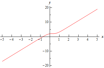
\[y\left( x \right) = 4x - \frac{{1 - 9\,{{\bf{e}}^{ - 4x\,}}}}{{1 + 3\,{{\bf{e}}^{ - 4x\,}}}}\]

Note that because exponentials exist everywhere and the denominator of the second term is always positive (because exponentials are always positive and adding a positive one onto that won’t change the fact that it’s positive) the interval of validity for this solution will be all real numbers.

Here is a graph of the solution.

Here is the substitution that we’ll need for this example.

\[v = 9y - x\hspace{0.25in}v' = 9y' - 1\]

Plugging this into our differential equation gives,

\[\begin{align*}\frac{1}{9}\left( {v' + 1} \right) & = {{\bf{e}}^v}\\ v' & = 9{{\bf{e}}^v} - 1\\ \frac{{dv}}{{9{{\bf{e}}^v} - 1}} & = dx\hspace{0.25in} \Rightarrow \hspace{0.25in}\frac{{{{\bf{e}}^{ - v}}\,dv}}{{9 - {{\bf{e}}^{ - v}}}} = dx\end{align*}\]

Note that we did a little rewrite on the separated portion to make the integrals go a little easier. By multiplying the numerator and denominator by \({{\bf{e}}^{ - v}}\) we can turn this into a fairly simply substitution integration problem. So, upon integrating both sides we get,

\[\ln \left( {9 - {{\bf{e}}^{ - v}}} \right) = x + c\]

Solving for \(v\) gives,

\[\begin{align*}9 - {{\bf{e}}^{ - v}} & = {{\bf{e}}^c}{{\bf{e}}^x} = c{{\bf{e}}^x}\\ {{\bf{e}}^{ - v}} & = 9 - c{{\bf{e}}^x}\\ v & = - \ln \left( {9 - c{{\bf{e}}^x}} \right)\end{align*}\]

Plugging the substitution back in and solving for \(y\) gives us,

\[y\left( x \right) = \frac{1}{9}\left( {x - \ln \left( {9 - c{{\bf{e}}^x}} \right)} \right)\]

Next, apply the initial condition and solve for \(c\).

\[0 = y\left( 0 \right) = - \frac{1}{9}\ln \left( {9 - c} \right)\hspace{0.25in} \Rightarrow \hspace{0.25in}c = 8\]

The solution is then,

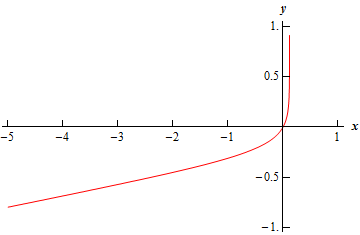
\[y\left( x \right) = \frac{1}{9}\left( {x - \ln \left( {9 - 8{{\bf{e}}^x}} \right)} \right)\]

Now, for the interval of validity we need to make sure that we only take logarithms of positive numbers as we’ll need to require that,

\[9 - 8{{\bf{e}}^x} > 0\hspace{0.25in} \Rightarrow \hspace{0.25in}{{\bf{e}}^x} < \frac{9}{8}\hspace{0.25in} \Rightarrow \hspace{0.25in}x < \ln \frac{9}{8} = 0.1178\]

Here is a graph of the solution.