Section 12.6 : Vector Functions
We first saw vector functions back when we were looking at the Equation of Lines. In that section we talked about them because we wrote down the equation of a line in \({\mathbb{R}^3}\) in terms of a vector function (sometimes called a vector-valued function). In this section we want to look a little closer at them and we also want to look at some vector functions in \({\mathbb{R}^3}\)other than lines.
A vector function is a function that takes one or more variables and returns a vector. We’ll spend most of this section looking at vector functions of a single variable as most of the places where vector functions show up here will be vector functions of single variables. We will however briefly look at vector functions of two variables at the end of this section.
A vector functions of a single variable in \({\mathbb{R}^2}\) and \({\mathbb{R}^3}\) have the form,
\[\vec r\left( t \right) = \left\langle {f\left( t \right),g\left( t \right)} \right\rangle \hspace{0.25in}\hspace{0.25in}\hspace{0.25in}\hspace{0.25in}\vec r\left( t \right) = \left\langle {f\left( t \right),g\left( t \right),h\left( t \right)} \right\rangle \]respectively, where \(f\left( t \right)\),\(g\left( t \right)\) and \(h\left( t \right)\) are called the component functions.
The main idea that we want to discuss in this section is that of graphing and identifying the graph given by a vector function. Before we do that however, we should talk briefly about the domain of a vector function. The domain of a vector function is the set of all \(t\)’s for which all the component functions are defined.
The first component is defined for all \(t\)’s. The second component is only defined for \(t < 4\). The third component is only defined for \(t \ge - 1\). Putting all of these together gives the following domain.
\[\left[ { - 1,4} \right)\]This is the largest possible interval for which all three components are defined.
Let’s now move into looking at the graph of vector functions. In order to graph a vector function all we do is think of the vector returned by the vector function as a position vector for points on the graph. Recall that a position vector, say \(\vec v = \left\langle {a,b,c} \right\rangle \), is a vector that starts at the origin and ends at the point \(\left( {a,b,c} \right)\).
So, in order to sketch the graph of a vector function all we need to do is plug in some values of \(t\) and then plot points that correspond to the resulting position vector we get out of the vector function.
Because it is a little easier to visualize things we’ll start off by looking at graphs of vector functions in \({\mathbb{R}^2}\).
- \(\vec r\left( t \right) = \left\langle {t,1} \right\rangle \)
- \(\vec r\left( t \right) = \left\langle {t,{t^3} - 10t + 7} \right\rangle \)
Okay, the first thing that we need to do is plug in a few values of \(t\) and get some position vectors. Here are a few,
\[\vec r\left( { - 3} \right) = \left\langle { - 3,1} \right\rangle \hspace{0.25in}\hspace{0.25in}\vec r\left( { - 1} \right) = \left\langle { - 1,1} \right\rangle \hspace{0.25in}\hspace{0.25in}\vec r\left( 2 \right) = \left\langle {2,1} \right\rangle \hspace{0.25in}\hspace{0.25in}\vec r\left( 5 \right) = \left\langle {5,1} \right\rangle \]So, what this tells us is that the following points are all on the graph of this vector function.
\[\left( { - 3,1} \right)\hspace{0.25in}\hspace{0.25in}\left( { - 1,1} \right)\hspace{0.25in}\hspace{0.25in}\left( {2,1} \right)\hspace{0.25in}\hspace{0.25in}\left( {5,1} \right)\]Here is a sketch of this vector function.
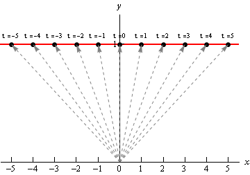
In this sketch we’ve included many more evaluations than just those above. Also note that we’ve put in the position vectors (in gray and dashed) so you can see how all this is working. Note however, that in practice the position vectors are generally not included in the sketch.
In this case it looks like we’ve got the graph of the line \(y = 1\).
b \(\vec r\left( t \right) = \left\langle {t,{t^3} - 10t + 7} \right\rangle \) Show Solution
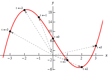
Here are a couple of evaluations for this vector function.
\[\vec r\left( { - 3} \right) = \left\langle { - 3,10} \right\rangle \hspace{0.25in}\vec r\left( { - 1} \right) = \left\langle { - 1,16} \right\rangle \hspace{0.25in}\vec r\left( 1 \right) = \left\langle {1, - 2} \right\rangle \hspace{0.25in}\vec r\left( 3 \right) = \left\langle {3,4} \right\rangle \]So, we’ve got a few points on the graph of this function. However, unlike the first part this isn’t really going to be enough points to get a good idea of this graph. In general, it can take quite a few function evaluations to get an idea of what the graph is and it’s usually easier to use a computer to do the graphing.
Here is a sketch of this graph. We’ve put in a few vectors/evaluations to illustrate them, but the reality is that we did have to use a computer to get a good sketch here.
Both of the vector functions in the above example were in the form,
\[\vec r\left( t \right) = \left\langle {t,g\left( t \right)} \right\rangle \]and what we were really sketching is the graph of \(y = g\left( x \right)\) as you probably caught onto. Let’s graph a couple of other vector functions that do not fall into this pattern.
- \(\vec r\left( t \right) = \left\langle {6\cos t,3\sin t} \right\rangle \)
- \(\vec r\left( t \right) = \left\langle {t - 2\sin t,{t^2}} \right\rangle \)
As we saw in the last part of the previous example it can really take quite a few function evaluations to really be able to sketch the graph of a vector function. Because of that we’ll be skipping all the function evaluations here and just giving the graph. The main point behind this set of examples is to not get you too locked into the form we were looking at above. The first part will also lead to an important idea that we’ll discuss after this example.
So, with that said here are the sketches of each of these.
a \(\vec r\left( t \right) = \left\langle {6\cos t,3\sin t} \right\rangle \) Show Solution
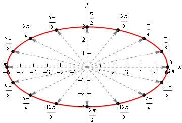
So, in this case it looks like we’ve got an ellipse.
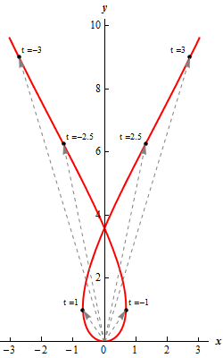
b \(\vec r\left( t \right) = \left\langle {t - 2\sin t,{t^2}} \right\rangle \) Show Solution
Here’s the sketch for this vector function.
Before we move on to vector functions in \({\mathbb{R}^3}\) let’s go back and take a quick look at the first vector function we sketched in the previous example, \(\vec r\left( t \right) = \left\langle {6\cos t,3\sin t} \right\rangle \). The fact that we got an ellipse here should not come as a surprise to you. We know that the first component function gives the \(x\) coordinate and the second component function gives the \(y\) coordinates of the point that we graph. If we strip these out to make this clear we get,
\[x = 6\cos t\hspace{0.25in}\hspace{0.25in}y = 3\sin t\]This should look familiar to you. Back when we were looking at Parametric Equations we saw that this was nothing more than one of the sets of parametric equations that gave an ellipse.
This is an important idea in the study of vector functions. Any vector function can be broken down into a set of parametric equations that represent the same graph. In general, the two dimensional vector function, \(\vec r\left( t \right) = \left\langle {f\left( t \right),g\left( t \right)} \right\rangle \), can be broken down into the parametric equations,
\[x = f\left( t \right)\hspace{0.25in}\hspace{0.25in}\hspace{0.25in}y = g\left( t \right)\]Likewise, a three dimensional vector function, \(\vec r\left( t \right) = \left\langle {f\left( t \right),g\left( t \right),h\left( t \right)} \right\rangle \), can be broken down into the parametric equations,
\[x = f\left( t \right)\hspace{0.25in}y = g\left( t \right)\hspace{0.25in}z = h\left( t \right)\]Do not get too excited about the fact that we’re now looking at parametric equations in \({\mathbb{R}^3}\). They work in exactly the same manner as parametric equations in \({\mathbb{R}^2}\) which we’re used to dealing with already. The only difference is that we now have a third component.
Let’s take a look at a couple of graphs of vector functions.
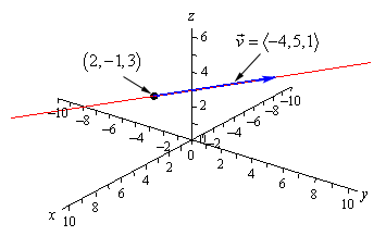
Notice that this is nothing more than a line. It might help if we rewrite it a little.
\[\vec r\left( t \right) = \left\langle {2, - 1,3} \right\rangle + t\left\langle { - 4,5,1} \right\rangle \]In this form we can see that this is the equation of a line that goes through the point \(\left( {2, - 1,3} \right)\) and is parallel to the vector \(\vec v = \left\langle { - 4,5,1} \right\rangle \).
To graph this line all that we need to do is plot the point and then sketch in the parallel vector. In order to get the sketch will assume that the vector is on the line and will start at the point in the line. To sketch in the line all we do this is extend the parallel vector into a line.
Here is a sketch.
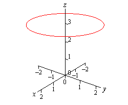
In this case to see what we’ve got for a graph let’s get the parametric equations for the curve.
\[x = 2\cos t\hspace{0.25in}\hspace{0.25in}y = 2\sin t\hspace{0.25in}\hspace{0.25in}z = 3\]If we ignore the \(z\) equation for a bit we’ll recall (hopefully) that the parametric equations for \(x\) and \(y\) give a circle of radius 2 centered on the origin (or about the \(z\)-axis since we are in \({\mathbb{R}^3}\)).
Now, all the parametric equations here tell us is that no matter what is going on in the graph all the \(z\) coordinates must be 3. So, we get a circle of radius 2 centered on the \(z\)-axis and at the level of \(z = 3\).
Here is a sketch.
Note that it is very easy to modify the above vector function to get a circle centered on the \(x\) or \(y\)-axis as well. For instance,
\[\vec r\left( t \right) = \left\langle {10\sin t, - 3,10\cos t} \right\rangle \]will be a circle of radius 10 centered on the \(y\)-axis and at \(y = - 3\). In other words, as long as two of the terms are a sine and a cosine (with the same coefficient) and the other is a fixed number then we will have a circle that is centered on the axis that is given by the fixed number.
Let’s take a look at a modification of this.
If this one had a constant in the \(z\) component we would have another circle. However, in this case we don’t have a constant. Instead we’ve got a \(t\) and that will change the curve. However, because the \(x\) and \(y\) component functions are still a circle in parametric equations our curve should have a circular nature to it in some way.
In fact, the only change is in the \(z\) component and as \(t\) increases the \(z\) coordinate will increase. Also, as \(t\) increases the \(x\) and \(y\) coordinates will continue to form a circle centered on the \(z\)-axis. Putting these two ideas together tells us that as we increase \(t\) the circle that is being traced out in the \(x\) and \(y\) directions should also be rising.
Here is a sketch of this curve.
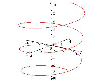
So, we’ve got a helix (or spiral, depending on what you want to call it) here.
As with circles the component that has the \(t\) will determine the axis that the helix rotates about. For instance,
\[\vec r\left( t \right) = \left\langle {t,6\cos t,6\sin t} \right\rangle \]is a helix that rotates around the \(x\)-axis.
Also note that if we allow the coefficients on the sine and cosine for both the circle and helix to be different we will get ellipses.
For example,
\[\vec r\left( t \right) = \left\langle {9\cos t,t,2\sin t} \right\rangle \]will be a helix that rotates about the \(y\)-axis and is in the shape of an ellipse.
There is a nice formula that we should derive before moving onto vector functions of two variables.
It is important to note here that we only want the equation of the line segment that starts at \(P\) and ends at \(Q\). We don’t want any other portion of the line and we do want the direction of the line segment preserved as we increase \(t\). With all that said, let’s not worry about that and just find the vector equation of the line that passes through the two points. Once we have this we will be able to get what we’re after.
So, we need a point on the line. We’ve got two and we will use \(P\). We need a vector that is parallel to the line and since we’ve got two points we can find the vector between them. This vector will lie on the line and hence be parallel to the line. Also, let’s remember that we want to preserve the starting and ending point of the line segment so let’s construct the vector using the same “orientation”.
\[\vec v = \left\langle {{x_2} - {x_1},{y_2} - {y_1},{z_2} - {z_1}} \right\rangle \]Using this vector and the point \(P\) we get the following vector equation of the line.
\[\vec r\left( t \right) = \left\langle {{x_1},{y_1},{z_1}} \right\rangle + t\left\langle {{x_2} - {x_1},{y_2} - {y_1},{z_2} - {z_1}} \right\rangle \]While this is the vector equation of the line, let’s rewrite the equation slightly.
\[\begin{align*}\vec r\left( t \right) & = \left\langle {{x_1},{y_1},{z_1}} \right\rangle + t\left\langle {{x_2},{y_2},{z_2}} \right\rangle - t\left\langle {{x_1},{y_1},{z_1}} \right\rangle \\ & = \left( {1 - t} \right)\left\langle {{x_1},{y_1},{z_1}} \right\rangle + t\left\langle {{x_2},{y_2},{z_2}} \right\rangle \end{align*}\]This is the equation of the line that contains the points \(P\) and \(Q\). We of course just want the line segment that starts at \(P\) and ends at \(Q\). We can get this by simply restricting the values of \(t\).
Notice that
\[\vec r\left( 0 \right) = \left\langle {{x_1},{y_1},{z_1}} \right\rangle \hspace{0.25in}\hspace{0.25in}\vec r\left( 1 \right) = \left\langle {{x_2},{y_2},{z_2}} \right\rangle \]So, if we restrict \(t\) to be between zero and one we will cover the line segment and we will start and end at the correct point.
So, the vector equation of the line segment that starts at \(P = \left( {{x_1},{y_1},{z_1}} \right)\) and ends at \(Q = \left( {{x_2},{y_2},{z_2}} \right)\) is,
\[\vec r\left( t \right) = \left( {1 - t} \right)\left\langle {{x_1},{y_1},{z_1}} \right\rangle + t\left\langle {{x_2},{y_2},{z_2}} \right\rangle \hspace{0.25in}\hspace{0.25in}0 \le t \le 1\]As noted briefly at the beginning of this section we can also have vector functions of two variables. In these cases the graphs of vector function of two variables are surfaces. So, to make sure that we don’t forget that let’s work an example with that as well.
First, notice that in this case the vector function will in fact be a function of two variables. This will always be the case when we are using vector functions to represent surfaces.
To identify the surface let’s go back to parametric equations.
\[x = x\hspace{0.25in}\hspace{0.25in}y = y\hspace{0.25in}\hspace{0.25in}\hspace{0.25in}z = {x^2} + {y^2}\]The first two are really only acknowledging that we are picking \(x\) and \(y\) for free and then determining \(z\) from our choices of these two. The last equation is the one that we want. We should recognize that function from the section on quadric surfaces. The third equation is the equation of an elliptic paraboloid and so the vector function represents an elliptic paraboloid.
As a final topic for this section let’s generalize the idea from the previous example and note that given any function of one variable (\(y = f\left( x \right)\) or \(x = h\left( y \right)\)) or any function of two variables (\(z = g\left( {x,y} \right)\),\(x = g\left( {y,z} \right)\), or \(y = g\left( {x,z} \right)\)) we can always write down a vector form of the equation.
For a function of one variable this will be,
\[\vec r\left( x \right) = x\,\vec i + f\left( x \right)\,\vec j\hspace{0.25in}\hspace{0.25in}\hspace{0.25in}\vec r\left( y \right) = h\left( y \right)\,\vec i + y\,\vec j\]and for a function of two variables the vector form will be,
\[\begin{array}{c}\vec r\left( {x,y} \right) = x\,\vec i + y{\kern 1pt} \vec j + g\left( {x,y} \right)\,\vec k\hspace{0.25in}\hspace{0.25in}\hspace{0.25in}\vec r\left( {y,z} \right) = g\left( {y,z} \right)\,\vec i + y{\kern 1pt} \vec j + z\,\vec k\\ \vec r\left( {x,z} \right) = x\,\vec i + g\left( {x,z} \right){\kern 1pt} \vec j + z\,\vec k\end{array}\]depending upon the original form of the function.
For example, the hyperbolic paraboloid \(y = 2{x^2} - 5{z^2}\) can be written as the following vector function.
\[\vec r\left( {x,z} \right) = x\,\vec i + \left( {2{x^2} - 5{z^2}} \right)\,\vec j + z\,\vec k\]This is a fairly important idea and we will be doing quite a bit of this kind of thing in Calculus III.