Section 12.1 : The 3-D Coordinate System
We’ll start the chapter off with a fairly short discussion introducing the 3-D coordinate system and the conventions that we’ll be using. We will also take a brief look at how the different coordinate systems can change the graph of an equation.
Let’s first get some basic notation out of the way. The 3-D coordinate system is often denoted by \({\mathbb{R}^3}\). Likewise, the 2-D coordinate system is often denoted by \({\mathbb{R}^2}\) and the 1-D coordinate system is denoted by \(\mathbb{R}\). Also, as you might have guessed then a general \(n\) dimensional coordinate system is often denoted by \({\mathbb{R}^n}\).
Next, let’s take a quick look at the basic coordinate system.
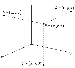
This is the standard placement of the axes in this class. It is assumed that only the positive directions are shown by the axes. If we need the negative axes for any reason we will put them in as needed.
Also note the various points on this sketch. The point \(P\) is the general point sitting out in 3-D space. If we start at \(P\) and drop straight down until we reach a \(z\)-coordinate of zero we arrive at the point \(Q\). We say that \(Q\) sits in the \(xy\)-plane. The \(xy\)-plane corresponds to all the points which have a zero \(z\)-coordinate. We can also start at \(P\) and move in the other two directions as shown to get points in the \(xz\)-plane (this is \(S\) with a \(y\)-coordinate of zero) and the \(yz\)-plane (this is \(R\) with an \(x\)-coordinate of zero).
Collectively, the \(xy\), \(xz\), and \(yz\)-planes are sometimes called the coordinate planes. In the remainder of this class you will need to be able to deal with the various coordinate planes so make sure that you can.
Also, the point \(Q\) is often referred to as the projection of \(P\) in the \(xy\)-plane. Likewise, \(R\) is the projection of \(P\) in the \(yz\)-plane and \(S\) is the projection of \(P\) in the \(xz\)-plane.
Many of the formulas that you are used to working with in \({\mathbb{R}^2}\) have natural extensions in \({\mathbb{R}^3}\). For instance, the distance between two points in \({\mathbb{R}^2}\) is given by,
\[d\left( {{P_1},{P_2}} \right) = \sqrt {{{\left( {{x_2} - {x_1}} \right)}^2} + {{\left( {{y_2} - {y_1}} \right)}^2}} \]While the distance between any two points in \({\mathbb{R}^3}\) is given by,
\[d\left( {{P_1},{P_2}} \right) = \sqrt {{{\left( {{x_2} - {x_1}} \right)}^2} + {{\left( {{y_2} - {y_1}} \right)}^2} + {{\left( {{z_2} - {z_1}} \right)}^2}} \]Likewise, the general equation for a circle with center \(\left( {h,k} \right)\) and radius \(r\) is given by,
\[{\left( {x - h} \right)^2} + {\left( {y - k} \right)^2} = {r^2}\]and the general equation for a sphere with center \(\left( {h,k,l} \right)\) and radius \(r\) is given by,
\[{\left( {x - h} \right)^2} + {\left( {y - k} \right)^2} + {\left( {z - l} \right)^2} = {r^2}\]With that said we do need to be careful about just translating everything we know about \({\mathbb{R}^2}\) into \({\mathbb{R}^3}\) and assuming that it will work the same way. A good example of this is in graphing to some extent. Consider the following example.
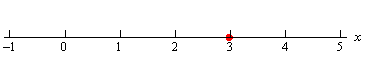
In \(\mathbb{R}\) we have a single coordinate system and so \(x = 3\) is a point in a 1-D coordinate system.
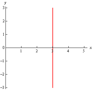
In \({\mathbb{R}^2}\) the equation \(x = 3\) tells us to graph all the points that are in the form \(\left( {3,y} \right)\). This is a vertical line in a 2-D coordinate system.
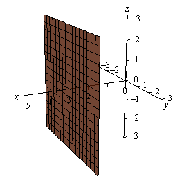
In \({\mathbb{R}^3}\) the equation \(x = 3\) tells us to graph all the points that are in the form \(\left( {3,y,z} \right)\). If you go back and look at the coordinate plane points this is very similar to the coordinates for the \(yz\)-plane except this time we have \(x = 3\) instead of \(x = 0\). So, in a 3-D coordinate system this is a plane that will be parallel to the \(yz\)-plane and pass through the \(x\)-axis at \(x = 3\).
Here is the graph of \(x = 3\) in \(\mathbb{R}\).
Here is the graph of \(x = 3\) in \({\mathbb{R}^2}\).
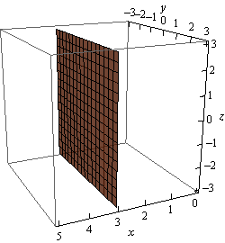
Finally, here is the graph of \(x = 3\) in \({\mathbb{R}^3}\). Note that we’ve presented this graph in two different styles. On the left we’ve got the traditional axis system that we’re used to seeing and on the right we’ve put the graph in a box. Both views can be convenient on occasion to help with perspective and so we’ll often do this with 3D graphs and sketches.
Note that at this point we can now write down the equations for each of the coordinate planes as well using this idea.
\[\begin{align*}z & = 0\hspace{0.25in}\hspace{0.25in}xy - {\mbox{plane}}\\ y & = 0\hspace{0.25in}\hspace{0.25in}xz - {\mbox{plane}}\\ x & = 0\hspace{0.25in}\hspace{0.25in}yz - {\mbox{plane}}\end{align*}\]Let’s take a look at a slightly more general example.
Note we had to throw out \(\mathbb{R}\) for this example since there are two variables which means that we can’t be in a 1-D space (1-D space has only one variable!).
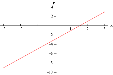
In \({\mathbb{R}^2}\) this is a line with slope 2 and a \(y\) intercept of -3.
However, in \({\mathbb{R}^3}\) this is not necessarily a line. Because we have not specified a value of \(z\) we are forced to let \(z\) take any value. This means that at any particular value of \(z\) we will get a copy of this line. So, the graph is then a vertical plane that lies over the line given by \(y = 2x - 3\) in the \(xy\)-plane.
Here is the graph in \({\mathbb{R}^2}\).
here is the graph in \({\mathbb{R}^3}\).
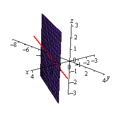
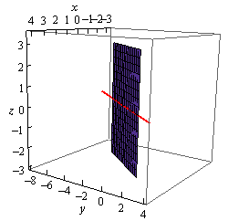
Notice that if we look to where the plane intersects the \(xy\)-plane we will get the graph of the line in \({\mathbb{R}^2}\) as noted in the above graph by the red line through the plane.
Let’s take a look at one more example of the difference between graphs in the different coordinate systems.
As with the previous example this won’t have a 1-D graph since there are two variables.
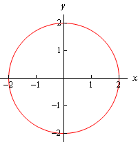
In \({\mathbb{R}^2}\) this is a circle centered at the origin with radius 2.
In \({\mathbb{R}^3}\) however, as with the previous example, this may or may not be a circle. Since we have not specified \(z\) in any way we must assume that \(z\) can take on any value. In other words, at any value of \(z\) this equation must be satisfied and so at any value \(z\) we have a circle of radius 2 centered on the z-axis. This means that we have a cylinder of radius 2 centered on the \(z\)-axis.
Here are the graphs for this example.
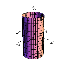
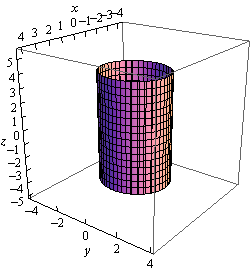
Notice that again, if we look to where the cylinder intersects the \(xy\)-plane we will again get the circle from \({\mathbb{R}^2}\).
We need to be careful with the last two examples. It would be tempting to take the results of these and say that we can’t graph lines or circles in \({\mathbb{R}^3}\) and yet that doesn’t really make sense. There is no reason for there to not be graphs of lines or circles in \({\mathbb{R}^3}\). Let’s think about the example of the circle. To graph a circle in \({\mathbb{R}^3}\) we would need to do something like \({x^2} + {y^2} = 4\) at \(z = 5\). This would be a circle of radius 2 centered on the \(z\)-axis at the level of \(z = 5\). So, as long as we specify a \(z\) we will get a circle and not a cylinder. We will see an easier way to specify circles in a later section.
We could do the same thing with the line from the second example. However, we will be looking at lines in more generality in the next section and so we’ll see a better way to deal with lines in \({\mathbb{R}^3}\) there.
The point of the examples in this section is to make sure that we are being careful with graphing equations and making sure that we always remember which coordinate system that we are in.
Another quick point to make here is that, as we’ve seen in the above examples, many graphs of equations in \({\mathbb{R}^3}\) are surfaces. That doesn’t mean that we can’t graph curves in \({\mathbb{R}^3}\). We can and will graph curves in \({\mathbb{R}^3}\) as well as we’ll see later in this chapter.