Section 2.9 : Euler's Method
Up to this point practically every differential equation that we’ve been presented with could be solved. The problem with this is that these are the exceptions rather than the rule. The vast majority of first order differential equations can’t be solved.
In order to teach you something about solving first order differential equations we’ve had to restrict ourselves down to the fairly restrictive cases of linear, separable, or exact differential equations or differential equations that could be solved with a set of very specific substitutions. Most first order differential equations however fall into none of these categories. In fact, even those that are separable or exact cannot always be solved for an explicit solution. Without explicit solutions to these it would be hard to get any information about the solution.
So, what do we do when faced with a differential equation that we can’t solve? The answer depends on what you are looking for. If you are only looking for long term behavior of a solution you can always sketch a direction field. This can be done without too much difficulty for some fairly complex differential equations that we can’t solve to get exact solutions.
The problem with this approach is that it’s only really good for getting general trends in solutions and for long term behavior of solutions. There are times when we will need something more. For instance, maybe we need to determine how a specific solution behaves, including some values that the solution will take. There are also a fairly large set of differential equations that are not easy to sketch good direction fields for.
In these cases, we resort to numerical methods that will allow us to approximate solutions to differential equations. There are many different methods that can be used to approximate solutions to a differential equation and in fact whole classes can be taught just dealing with the various methods. We are going to look at one of the oldest and easiest to use here. This method was originally devised by Euler and is called, oddly enough, Euler’s Method.
Let’s start with a general first order IVP
\[\begin{equation}\frac{{dy}}{{dt}} = f\left( {t,y} \right)\hspace{0.25in}y\left( {{t_0}} \right) = {y_0}\label{eq:eq1}\end{equation}\]where \(f(t,y)\) is a known function and the values in the initial condition are also known numbers. From the second theorem in the Intervals of Validity section we know that if \(f\) and \(f_{y}\) are continuous functions then there is a unique solution to the IVP in some interval surrounding \(t = {t_0}\). So, let’s assume that everything is nice and continuous so that we know that a solution will in fact exist.
We want to approximate the solution to \(\eqref{eq:eq1}\) near \(t = {t_0}\). We’ll start with the two pieces of information that we do know about the solution. First, we know the value of the solution at \(t = {t_0}\) from the initial condition. Second, we also know the value of the derivative at \(t = {t_0}\). We can get this by plugging the initial condition into \(f(t,y)\) into the differential equation itself. So, the derivative at this point is.
\[{\left. {\frac{{dy}}{{dt}}} \right|_{t = {t_0}}} = f\left( {{t_0},{y_0}} \right)\]Now, recall from your Calculus I class that these two pieces of information are enough for us to write down the equation of the tangent line to the solution at \(t = {t_0}\). The tangent line is
\[y = {y_0} + f\left( {{t_0},{y_0}} \right)\left( {t - {t_0}} \right)\]Take a look at the figure below
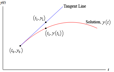
If \(t_{1}\) is close enough to \(t_{0}\) then the point \(y_{1}\) on the tangent line should be fairly close to the actual value of the solution at \(t_{1}\), or \(y(t_{1})\). Finding \(y_{1}\) is easy enough. All we need to do is plug \(t_{1}\) in the equation for the tangent line.
\[{y_1} = {y_0} + f\left( {{t_0},{y_0}} \right)\left( {{t_1} - {t_0}} \right)\]Now, we would like to proceed in a similar manner, but we don’t have the value of the solution at \(t_{1}\) and so we won’t know the slope of the tangent line to the solution at this point. This is a problem. We can partially solve it however, by recalling that \(y_{1}\) is an approximation to the solution at \(t_{1}\). If \(y_{1}\) is a very good approximation to the actual value of the solution then we can use that to estimate the slope of the tangent line at \(t_{1}\).
So, let’s hope that \(y_{1}\) is a good approximation to the solution and construct a line through the point (\(t_{1}, y_{1}\)) that has slope \(f(t_{1}, y_{1}\)). This gives
\[y = {y_1} + f\left( {{t_1},{y_1}} \right)\left( {t - {t_1}} \right)\]Now, to get an approximation to the solution at \(t=t_{2}\) we will hope that this new line will be fairly close to the actual solution at \(t_{2}\) and use the value of the line at \(t_{2}\) as an approximation to the actual solution. This gives.
\[{y_2} = {y_1} + f\left( {{t_1},{y_1}} \right)\left( {{t_2} - {t_1}} \right)\]We can continue in this fashion. Use the previously computed approximation to get the next approximation. So,
\[\begin{align*}{y_3} & = {y_2} + f\left( {{t_2},{y_2}} \right)\left( {{t_3} - {t_2}} \right)\\ {y_4} & = {y_3} + f\left( {{t_3},{y_3}} \right)\left( {{t_4} - {t_3}} \right)\\ & etc.\end{align*}\]In general, if we have \(t_{n}\) and the approximation to the solution at this point, \(y_{n}\), and we want to find the approximation at \(t_{n+1}\) all we need to do is use the following.
\[{y_{n + 1}} = {y_n} + f\left( {{t_n},{y_n}} \right) \cdot \left( {{t_{n + 1}} - {t_n}} \right)\]If we define \({f_n} = f\left( {{t_n},{y_n}} \right)\) we can simplify the formula to
\[\begin{equation}{y_{n + 1}} = {y_n} + {f_n} \cdot \left( {{t_{n + 1}} - {t_n}} \right)\label{eq:eq2}\end{equation}\]Often, we will assume that the step sizes between the points \(t_{0}\) , \(t_{1}\) , \(t_{2}\) , … are of a uniform size of \(h\). In other words, we will often assume that
\[{t_{n + 1}} - {t_n} = h\]This doesn’t have to be done and there are times when it’s best that we not do this. However, if we do the formula for the next approximation becomes.
\[\begin{equation}{y_{n + 1}} = {y_n} + h\,{f_n}\label{eq:eq3}\end{equation}\]So, how do we use Euler’s Method? It’s fairly simple. We start with \(\eqref{eq:eq1}\) and decide if we want to use a uniform step size or not. Then starting with \((t_{0}, y_{0})\) we repeatedly evaluate \(\eqref{eq:eq2}\) or \(\eqref{eq:eq3}\) depending on whether we chose to use a uniform step size or not. We continue until we’ve gone the desired number of steps or reached the desired time. This will give us a sequence of numbers \(y_{1}\) , \(y_{2}\) , \(y_{3}\) , … \(y_{n}\) that will approximate the value of the actual solution at \(t_{1}\) , \(t_{2}\) , \(t_{3}\) , … \(t_{n}\).
What do we do if we want a value of the solution at some other point than those used here? One possibility is to go back and redefine our set of points to a new set that will include the points we are after and redo Euler’s Method using this new set of points. However, this is cumbersome and could take a lot of time especially if we had to make changes to the set of points more than once.
Another possibility is to remember how we arrived at the approximations in the first place. Recall that we used the tangent line
\[y = {y_0} + f\left( {{t_0},{y_0}} \right)\left( {t - {t_0}} \right)\]to get the value of \(y_{1}\). We could use this tangent line as an approximation for the solution on the interval \([t_{0}, t_{1}]\). Likewise, we used the tangent line
\[y = {y_1} + f\left( {{t_1},{y_1}} \right)\left( {t - {t_1}} \right)\]to get the value of \(y_{2}\). We could use this tangent line as an approximation for the solution on the interval \([t_{1}, t_{2}]\). Continuing in this manner we would get a set of lines that, when strung together, should be an approximation to the solution as a whole.
In practice you would need to write a computer program to do these computations for you. In most cases the function \(f(t,y)\) would be too large and/or complicated to use by hand and in most serious uses of Euler’s Method you would want to use hundreds of steps which would make doing this by hand prohibitive. So, here is a bit of pseudo-code that you can use to write a program for Euler’s Method that uses a uniform step size, \(h\).
- define \(f\left( {t,y} \right)\).
- input \(t_{0}\) and \(y_{0}\).
- input step size, \(h\) and the number of steps, \(n\).
- for \(j\) from 1 to \(n\) do
- \(m = f(t_{0}, y_{0})\)
- \(y_{1} = y_{0} + h*m\)
- \(t_{1} = t_{0} + h\)
- Print \(t_{1}\) and \(y_{1}\)
- \(t_{0} = t_{1}\)
- \(y_{0} = y_{1}\)
- end
The pseudo-code for a non-uniform step size would be a little more complicated, but it would essentially be the same.
So, let’s take a look at a couple of examples. We’ll use Euler’s Method to approximate solutions to a couple of first order differential equations. The differential equations that we’ll be using are linear first order differential equations that can be easily solved for an exact solution. Of course, in practice we wouldn’t use Euler’s Method on these kinds of differential equations, but by using easily solvable differential equations we will be able to check the accuracy of the method. Knowing the accuracy of any approximation method is a good thing. It is important to know if the method is liable to give a good approximation or not.
Use Euler’s Method with a step size of \(h = 0.1\) to find approximate values of the solution at \(t\) = 0.1, 0.2, 0.3, 0.4, and 0.5. Compare them to the exact values of the solution at these points.
This is a fairly simple linear differential equation so we’ll leave it to you to check that the solution is
\[y\left( t \right) = 1 + \frac{1}{2}{{\bf{e}}^{ - 4t}} - \frac{1}{2}{{\bf{e}}^{ - 2t}}\]In order to use Euler’s Method we first need to rewrite the differential equation into the form given in \(\eqref{eq:eq1}\).
\[y' = 2 - {{\bf{e}}^{ - 4t}} - 2y\]From this we can see that \(f\left( {t,y} \right) = 2 - {{\bf{e}}^{ - 4t}} - 2y\). Also note that \(t_{0} = 0\) and \(y_{0} = 1\). We can now start doing some computations.
\[\begin{align*}{f_0} &= f\left( {0,1} \right) = 2 - {{\bf{e}}^{ - 4\left( 0 \right)}} - 2\left( 1 \right) = - 1\\ {y_1} & = {y_0} + h\,{f_0} = 1 + \left( {0.1} \right)\left( { - 1} \right) = 0.9\end{align*}\]So, the approximation to the solution at \(t_{1} = 0.1\) is \(y_{1} = 0.9\).
At the next step we have
\[\begin{align*}{f_1} & = f\left( {0.1,0.9} \right) = 2 - {{\bf{e}}^{ - 4\left( {0.1} \right)}} - 2\left( {0.9} \right) = - \,0.470320046\\ {y_2} & = {y_1} + h\,{f_1} = 0.9 + \left( {0.1} \right)\left( { - \,0.470320046} \right) = 0.852967995\end{align*}\]Therefore, the approximation to the solution at \(t_{2} = 0.2\) is \(y_{2} = 0.852967995\).
I’ll leave it to you to check the remainder of these computations.
\[\begin{align*}{f_2} & = - 0.155264954 & \hspace{0.25in}{y_3} & = 0.837441500\\ {f_3} & = 0.023922788 & \hspace{0.25in}{y_4} & = 0.839833779\\ {f_4} & = 0.1184359245 & \hspace{0.25in}{y_5}& = 0.851677371\end{align*}\]Here’s a quick table that gives the approximations as well as the exact value of the solutions at the given points.
| Time, \(t_{n}\) | Approximation | Exact | Error |
|---|---|---|---|
| \(t_{0} = 0\) | \(y_{0} =1\) | \(y(0) = 1\) | 0 % |
| \(t_{1} = 0.1\) | \(y_{1} =0.9\) | \(y(0.1) = 0.925794646\) | 2.79 % |
| \(t_{2} = 0.2\) | \(y_{2} =0.852967995\) | \(y(0.2) = 0.889504459\) | 4.11 % |
| \(t_{3} = 0.3\) | \(y_{3} =0.837441500\) | \(y(0.3) = 0.876191288\) | 4.42 % |
| \(t_{4} = 0.4\) | \(y_{4} =0.839833779\) | \(y(0.4) = 0.876283777\) | 4.16 % |
| \(t_{5} = 0.5\) | \(y_{5} =0.851677371\) | \(y(0.5) = 0.883727921\) | 3.63 % |
We’ve also included the error as a percentage. It’s often easier to see how well an approximation does if you look at percentages. The formula for this is,
\[\mbox{percent error} = \frac{{\left| {\mbox{exact} - \mbox{approximate}} \right|}}{{\mbox{exact}}} \times 100\]We used absolute value in the numerator because we really don’t care at this point if the approximation is larger or smaller than the exact. We’re only interested in how close the two are.
The maximum error in the approximations from the last example was 4.42%, which isn’t too bad, but also isn’t all that great of an approximation. So, provided we aren’t after very accurate approximations this didn’t do too badly. This kind of error is generally unacceptable in almost all real applications however. So, how can we get better approximations?
Recall that we are getting the approximations by using a tangent line to approximate the value of the solution and that we are moving forward in time by steps of \(h\). So, if we want a more accurate approximation, then it seems like one way to get a better approximation is to not move forward as much with each step. In other words, take smaller \(h\)’s.
Below are two tables, one gives approximations to the solution and the other gives the errors for each approximation. We’ll leave the computational details to you to check.
| Approximations | ||||||
| Time | Exact | \(h = 0.1\) | \(h = 0.05\) | \(h = 0.01\) | \(h = 0.005\) | \(h = 0.001\) |
|---|---|---|---|---|---|---|
| \(t\) = 1 | 0.9414902 | 0.9313244 | 0.9364698 | 0.9404994 | 0.9409957 | 0.9413914 |
| \(t\) = 2 | 0.9910099 | 0.9913681 | 0.9911126 | 0.9910193 | 0.9910139 | 0.9910106 |
| \(t\) = 3 | 0.9987637 | 0.9990501 | 0.9988982 | 0.9987890 | 0.9987763 | 0.9987662 |
| \(t\) = 4 | 0.9998323 | 0.9998976 | 0.9998657 | 0.9998390 | 0.9998357 | 0.9998330 |
| \(t\) = 5 | 0.9999773 | 0.9999890 | 0.9999837 | 0.9999786 | 0.9999780 | 0.9999774 |
| Percentage Errors | |||||
| Time | \(h = 0.1\) | \(h = 0.05\) | \(h = 0.01\) | \(h = 0.005\) | \(h = 0.001\) |
|---|---|---|---|---|---|
| \(t\) = 1 | 1.08 % | 0.53 % | 0.105 % | 0.053 % | 0.0105 % |
| \(t\) = 2 | 0.036 % | 0.010 % | 0.00094 % | 0.00041 % | 0.0000703 % |
| \(t\) = 3 | 0.029 % | 0.013 % | 0.0025 % | 0.0013 % | 0.00025 % |
| \(t\) = 4 | 0.0065 % | 0.0033 % | 0.00067 % | 0.00034 % | 0.000067 % |
| \(t\) = 5 | 0.0012 % | 0.00064 % | 0.00013 % | 0.000068 % | 0.000014 % |
We can see from these tables that decreasing \(h\) does in fact improve the accuracy of the approximation as we expected.
There are a couple of other interesting things to note from the data. First, notice that in general, decreasing the step size, \(h\), by a factor of 10 also decreased the error by about a factor of 10 as well.
Also, notice that as \(t\) increases the approximation actually tends to get better. This isn’t the case completely as we can see that in all but the first case the \(t\) = 3 error is worse than the error at \(t\) = 2, but after that point, it only gets better. This should not be expected in general. In this case this is more a function of the shape of the solution. Below is a graph of the solution (the line) as well as the approximations (the dots) for \(h = 0.1\).
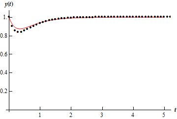
Notice that the approximation is worst where the function is changing rapidly. This should not be too surprising. Recall that we’re using tangent lines to get the approximations and so the value of the tangent line at a given \(t\) will often be significantly different than the function due to the rapidly changing function at that point.
Also, in this case, because the function ends up fairly flat as \(t\) increases, the tangents start looking like the function itself and so the approximations are very accurate. This won’t always be the case of course.
Let’s take a look at one more example.
Use Euler’s Method to find the approximation to the solution at \(t = 1\), \(t = 2\), \(t = 3\), \(t = 4\), and \(t = 5\). Use \(h = 0.1\), \(h = 0.05\), \(h = 0.01\), \(h = 0.005\), and \(h = 0.001\) for the approximations.
We’ll leave it to you to check the details of the solution process. The solution to this linear first order differential equation is.
\[y\left( t \right) = {{\bf{e}}^{\frac{t}{2}}}\sin \left( {5t} \right)\]Here are two tables giving the approximations and the percentage error for each approximation.
| Approximations | ||||||
| Time | Exact | \(h = 0.1\) | \(h = 0.05\) | \(h = 0.01\) | \(h = 0.005\) | \(h = 0.001\) |
|---|---|---|---|---|---|---|
| \(t\) = 1 | -1.58100 | -0.97167 | -1.26512 | -1.51580 | -1.54826 | -1.57443 |
| \(t\) = 2 | -1.47880 | 0.65270 | -0.34327 | -1.23907 | -1.35810 | -1.45453 |
| \(t\) = 3 | 2.91439 | 7.30209 | 5.34682 | 3.44488 | 3.18259 | 2.96851 |
| \(t\) = 4 | 6.74580 | 15.56128 | 11.84839 | 7.89808 | 7.33093 | 6.86429 |
| \(t\) = 5 | -1.61237 | 21.95465 | 12.24018 | 1.56056 | 0.0018864 | -1.28498 |
| Percentage Errors | |||||
| Time | \(h = 0.1\) | \(h = 0.05\) | \(h = 0.01\) | \(h = 0.005\) | \(h = 0.001\) |
|---|---|---|---|---|---|
| \(t\) = 1 | 38.54 % | 19.98 % | 4.12 % | 2.07 % | 0.42 % |
| \(t\) = 2 | 144.14 % | 76.79 % | 16.21 % | 8.16 % | 1.64 % |
| \(t\) = 3 | 150.55 % | 83.46 % | 18.20 % | 9.20 % | 1.86 % |
| \(t\) = 4 | 130.68 % | 75.64 % | 17.08 % | 8.67 % | 1.76 % |
| \(t\) = 5 | 1461.63 % | 859.14 % | 196.79 % | 100.12 % | 20.30 % |
So, with this example Euler’s Method does not do nearly as well as it did on the first IVP. Some of the observations we made in Example 2 are still true however. Decreasing the size of \(h\) decreases the error as we saw with the last example and would expect to happen. Also, as we saw in the last example, decreasing \(h\) by a factor of 10 also decreases the error by about a factor of 10.
However, unlike the last example increasing \(t\) sees an increasing error. This behavior is fairly common in the approximations. We shouldn’t expect the error to decrease as \(t\) increases as we saw in the last example. Each successive approximation is found using a previous approximation. Therefore, at each step we introduce error and so approximations should, in general, get worse as \(t\) increases.
Below is a graph of the solution (the line) as well as the approximations (the dots) for \(h\) = 0.05.
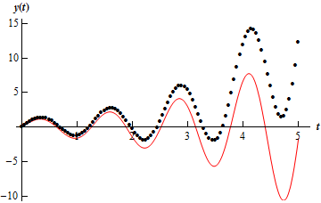
As we can see the approximations do follow the general shape of the solution, however, the error is clearly getting much worse as \(t\) increases.
So, Euler’s method is a nice method for approximating fairly nice solutions that don’t change rapidly. However, not all solutions will be this nicely behaved. There are other approximation methods that do a much better job of approximating solutions. These are not the focus of this course however, so I’ll leave it to you to look further into this field if you are interested.
Also notice that we don’t generally have the actual solution around to check the accuracy of the approximation. We generally try to find bounds on the error for each method that will tell us how well an approximation should do. These error bounds are again not really the focus of this course, so I’ll leave these to you as well if you’re interested in looking into them.