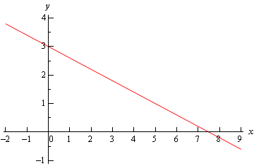
This is a line in the slope intercept form

\[y = mx + b\]

In this case the line has a \(y\) intercept of \(\left(0,b\right)\) and a slope of \(m\). Recall that slope can be thought of as

\[m = \frac{{{\rm{rise}}}}{{{\rm{run}}}}\]

Note that if the slope is negative we tend to think of the rise as a fall.

The slope allows us to get a second point on the line. Once we have any point on the line and the slope we move right by run and up/down by rise depending on the sign. This will be a second point on the line.

In this case we know \(\left(0,3\right)\) is a point on the line and the slope is \( - \frac{2}{5}\). So starting at \(\left(0,3\right)\) we’ll move 5 to the right (i.e. \(0 \to 5\)) and down 2 (i.e. \(3 \to 1\)) to get \(\left(5,1\right)\) as a second point on the line. Once we’ve got two points on a line all we need to do is plot the two points and connect them with a line.

Here’s the sketch for this line.

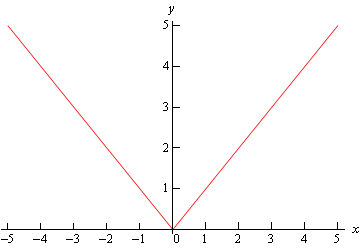
There really isn’t much to this problem outside of reminding ourselves of what absolute value is. Recall that the absolute value function is defined as,

\[\left| x \right| = \left\{ {\begin{array}{rl}x & {{\mbox{if }}x \ge 0}\\{ - x} & {{\mbox{if }}x < 0}\end{array}} \right.\]

The graph is then,

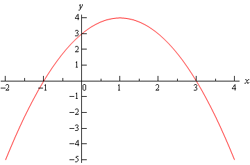
This is a parabola in the general form.

\[f\left( x \right) = a{x^2} + bx + c\]

In this form, the \(x\)-coordinate of the vertex (the highest or lowest point on the parabola) is \(x = - \frac{b}{{2a}}\) and the \(y\)-coordinate is \(y = f\left( { - \frac{b}{{2a}}} \right)\). So, for our parabola the coordinates of the vertex will be.

\[\begin{align*}x & = - \frac{2}{{2\left( { - 1} \right)}} = 1\\ y & = f\left( 1 \right) = - {\left( 1 \right)^2} + 2\left( 1 \right) + 3 = 4\end{align*}\]

So, the vertex for this parabola is \(\left(1,4\right)\).

We can also determine which direction the parabola opens from the sign of \(a\). If \(a\) is positive the parabola opens up and if \(a\) is negative the parabola opens down. In our case the parabola opens down.

Now, because the vertex is above the \(x\)-axis and the parabola opens down we know that we’ll have \(x\)-intercepts (i.e. values of \(x\) for which we’ll have \(f\left( x \right) = 0\)) on this graph. So, we’ll solve the following.

\[\begin{align*} - {x^2} + 2x + 3 & = 0\\ {x^2} - 2x - 3 & = 0\\ \left( {x - 3} \right)\left( {x + 1} \right) & = 0\end{align*}\]

So, we will have \(x\)-intercepts at \(x = - 1\) and \(x = 3\). Notice that to make our life easier in the solution process we multiplied everything by -1 to get the coefficient of the \({x^2}\) positive. This made the factoring easier.

Here’s a sketch of this parabola.

Most people come out of an Algebra class capable of dealing with functions in the form \(y = f(x)\). However, many functions that you will have to deal with in a Calculus class are in the form \(x = f(y)\) and can only be easily worked with in that form. So, you need to get used to working with functions in this form.

The nice thing about these kinds of function is that if you can deal with functions in the form \(y = f(x)\) then you can deal with functions in the form \(x = f(y)\) even if you aren’t that familiar with them.

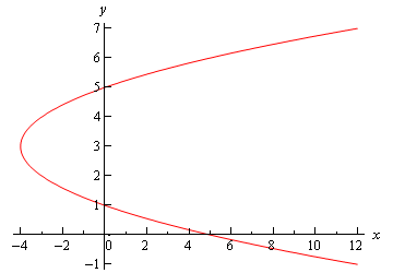
Let’s first consider the equation.

\[y = {x^2} - 6x + 5\]

This is a parabola that opens up and has a vertex of \(\left(3,-4\right)\), as we know from our work in the previous example.

For our function we have essentially the same equation except the \(x\) and \(y\)’s are switched around. In other words, we have a parabola in the form,

\[x = a{y^2} + by + c\]

This is the general form of this kind of parabola and this will be a parabola that opens left or right depending on the sign of \(a\). The \(y\)-coordinate of the vertex is given by \(y = - \frac{b}{{2a}}\) and we find the \(x\)-coordinate by plugging this into the equation. So, you can see that this is very similar to the type of parabola that you’re already used to dealing with.

Now, let’s get back to the example. Our function is a parabola that opens to the right (\(a\) is positive) and has a vertex at \(\left(-4,3\right)\). The vertex is to the left of the \(y\)-axis and opens to the right so we’ll need the \(y\)-intercepts (i.e. values of \(y\) for which we’ll have \(f\left( y \right) = 0\))). We find these just like we found ­\(x\)-intercepts in the previous problem.

\[\begin{align*}{y^2} - 6y + 5 & = 0\\ \left( {y - 5} \right)\left( {y - 1} \right) & = 0\end{align*}\]

So, our parabola will have ­\(y\)-intercepts at \(y = 1\) and \(y = 5\). Here’s a sketch of the graph.

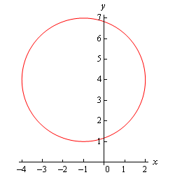
To determine just what kind of graph we’ve got here we need to complete the square on both the \(x\) and the \(y\).

\[\begin{align*}{x^2} + 2x + {y^2} - 8y + 8 & = 0\\ {x^2} + 2x + 1 - 1 + {y^2} - 8y + 16 - 16 + 8 & = 0\\ {\left( {x + 1} \right)^2} + {\left( {y - 4} \right)^2} & = 9\end{align*}\]

Recall that to complete the square we take the half of the coefficient of the \(x\) (or the \(y\)), square this and then add and subtract it to the equation.

Upon doing this we see that we have a circle and it’s now written in standard form.

\[{\left( {x - h} \right)^2} + {\left( {y - k} \right)^2} = {r^2}\]

When circles are in this form we can easily identify the center \(\left(h, k\right)\) and radius \(r\). Once we have these we can graph the circle simply by starting at the center and moving right, left, up and down by \(r\) to get the rightmost, leftmost, top most and bottom most points respectively.

Our circle has a center at \(\left(-1, 4\right)\) and a radius of 3. Here’s a sketch of this circle.

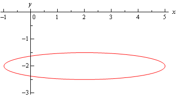
This is an ellipse. The standard form of the ellipse is

\[\frac{{{{\left( {x - h} \right)}^2}}}{{{a^2}}} + \frac{{{{\left( {y - k} \right)}^2}}}{{{b^2}}} = 1\]

This is an ellipse with center \(\left(h, k\right)\) and the right most and left most points are a distance of \(a\) away from the center and the top most and bottom most points are a distance of \(b\) away from the center.

The ellipse for this problem has center \(\left(2, -2\right)\) and has \(a = 3\) and \(b = \frac{1}{2}\). Note that to get the \(b\) we’re really rewriting the equation as,

\[\frac{{{\left( x-2 \right)}^{2}}}{9}+\frac{{{\left( y+2 \right)}^{2}}}{{}^{1}/{}_{4}}=1\]

to get it into standard from.

Here’s a sketch of the ellipse.

This is a hyperbola. There are actually two standard forms for a hyperbola. Here are the basics for each form.

Form	\(\displaystyle \frac{{{{\left( {x - h} \right)}^2}}}{{{a^2}}} - \frac{{{{\left( {y - k} \right)}^2}}}{{{b^2}}} = 1\)	\(\displaystyle \frac{{{{\left( {y - k} \right)}^2}}}{{{b^2}}} - \frac{{{{\left( {x - h} \right)}^2}}}{{{a^2}}} = 1\)
Center	\(\left(h, k\right)\)	\(\left(h, k\right)\)
Opens	Opens right and left	Opens up and down
Vertices	\(a\) units right and left of center	\(b\) units up and down from center
Slope of Asymptotes	\(\displaystyle \pm \frac{b}{a}\)	\(\displaystyle \pm \frac{b}{a}\)

So, what does all this mean? First, notice that one of the terms is positive and the other is negative. This will determine which direction the two parts of the hyperbola open. If the \(x\) term is positive the hyperbola opens left and right. Likewise, if the \(y\) term is positive the parabola opens up and down.

Both have the same “center”. Note that hyperbolas don’t really have a center in the sense that circles and ellipses have centers. The center is the starting point in graphing a hyperbola. It tells us how to get to the vertices and how to get the asymptotes set up.

The asymptotes of a hyperbola are two lines that intersect at the center and have the slopes listed above. As you move farther out from the center the graph will get closer and closer to the asymptotes.

For the equation listed here the hyperbola will open left and right. Its center is \(\left(-1, 2\right)\). The two vertices are \(\left(-4, 2\right)\) and \(\left(2, 2\right)\). The asymptotes will have slopes \( \pm \frac{2}{3}\).

Here is a sketch of this hyperbola. Note that the asymptotes are denoted by the two dashed lines.

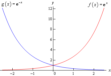
There really isn’t a lot to this problem other than making sure that both of these exponentials are graphed somewhere.

These will both show up with some regularity in later sections and their behavior as \(x\) goes to both plus and minus infinity will be needed and from this graph we can clearly see this behavior.

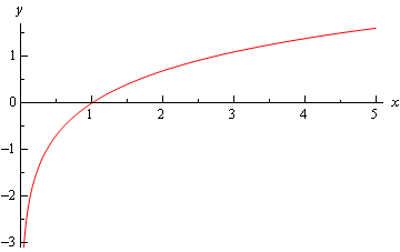
This has already been graphed once in this review, but this puts it here with all the other “important” graphs.

This one is fairly simple, we just need to make sure that we can graph it when need be.

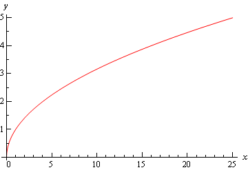
Remember that the domain of the square root function is \(x \ge 0\).

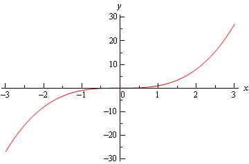
Again, there really isn’t much to this other than to make sure it’s been graphed somewhere so we can say we’ve done it.

There really isn’t a whole lot to this one. Here’s the graph for \( - 4\pi \le x \le 4\pi \).

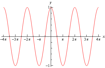
Let’s also note here that we can put all values of \(x\) into cosine (which won’t be the case for most of the trig functions) and so the domain is all real numbers. Also note that

\[ - 1 \le \cos \left( x \right) \le 1\]

It is important to notice that cosine will never be larger than 1 or smaller than -1. This will be useful on occasion in a calculus class. In general we can say that

\[ - R \le R\cos \left( {\omega \,x} \right) \le R\]

As with the previous problem there really isn’t a lot to do other than graph it. Here is the graph for \( - 4\pi \le x \le 4\pi \).

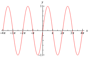
From this graph we can see that sine has the same range that cosine does. In general

\[ - R \le R\sin \left( {\omega \,x} \right) \le R\]

As with cosine, sine itself will never be larger than 1 and never smaller than -1. Also the domain of sine is all real numbers.

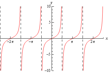
In the case of tangent we have to be careful when plugging \(x\)’s in since tangent doesn’t exist wherever cosine is zero (remember that \(\tan x = \frac{{\sin x}}{{\cos x}}\)). Tangent will not exist at

\[x = \cdots , - \frac{{5\pi }}{2}, - \frac{{3\pi }}{2}, - \frac{\pi }{2},\frac{\pi }{2},\frac{{3\pi }}{2},\frac{{5\pi }}{2}, \ldots \]

and the graph will have asymptotes at these points. Here is the graph of tangent on the range \( - \frac{{5\pi }}{2} < x < \frac{{5\pi }}{2}\).

As with tangent we will have to avoid \(x\)’s for which cosine is zero (remember that \(\sec x = \frac{1}{{\cos x}}\)). Secant will not exist at

\[x = \cdots , - \frac{{5\pi }}{2}, - \frac{{3\pi }}{2}, - \frac{\pi }{2},\frac{\pi }{2},\frac{{3\pi }}{2},\frac{{5\pi }}{2}, \ldots \]

and the graph will have asymptotes at these points. Here is the graph of secant on the range \( - \frac{{5\pi }}{2} < x < \frac{{5\pi }}{2}\).

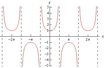
Notice that the graph is always greater than 1 or less than -1. This should not be terribly surprising. Recall that \[ - 1 \le \cos \left( x \right) \le 1\]. So, one divided by something less than one will be greater than 1. Also, \({}^{1}/{}_{\pm 1}=\pm 1\) and so we get the following ranges for secant.

\[\sec \left( {\omega \,x} \right) \ge 1\hspace{0.5in}{\rm{and}}\hspace{0.5in}\sec \left( {\omega \,x} \right) \le - 1\]