Section 15.3 : Double Integrals over General Regions
In the previous section we looked at double integrals over rectangular regions. The problem with this is that most of the regions are not rectangular so we need to now look at the following double integral,
\[\iint\limits_{D}{{f\left( {x,y} \right)\,dA}}\]where \(D\) is any region.
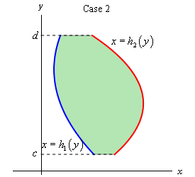
There are two types of regions that we need to look at. Here is a sketch of both of them.
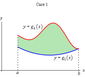
We will often use set builder notation to describe these regions. Here is the definition for the region in Case 1
\[D = \left\{ {\left( {x,y} \right)|a \le x \le b,\,\,{g_1}\left( x \right) \le y \le {g_2}\left( x \right)} \right\}\]and here is the definition for the region in Case 2.
\[D = \left\{ {\left( {x,y} \right)|{h_1}\left( y \right) \le x \le {h_2}\left( y \right),\,c \le y \le d} \right\}\]This notation is really just a fancy way of saying we are going to use all the points, \(\left( {x,y} \right)\), in which both of the coordinates satisfy the two given inequalities.
The double integral for both of these cases are defined in terms of iterated integrals as follows.
In Case 1 where \(D = \left\{ {\left( {x,y} \right)|a \le x \le b,\,\,{g_1}\left( x \right) \le y \le {g_2}\left( x \right)} \right\}\) the integral is defined to be,
\[\iint\limits_{D}{{f\left( {x,y} \right)\,dA}} = \int_{{\,a}}^{{\,b}}{{\int_{{{g_{\,1}}\left( x \right)}}^{{{g_{\,2}}\left( x \right)}}{{f\left( {x,y} \right)\,dy}}\,dx}}\]In Case 2 where \(D = \left\{ {\left( {x,y} \right)|{h_1}\left( y \right) \le x \le {h_2}\left( y \right),\,c \le y \le d} \right\}\) the integral is defined to be,
\[\iint\limits_{D}{{f\left( {x,y} \right)\,dA}} = \int_{{\,c}}^{{\,d}}{{\int_{{h{\,_1}\left( y \right)}}^{{{h_{\,2}}\left( y \right)}}{{f\left( {x,y} \right)\,dx}}\,dy}}\]Here are some properties of the double integral that we should go over before we actually do some examples. Note that all three of these properties are really just extensions of properties of single integrals that have been extended to double integrals.
Properties
- \(\displaystyle \iint\limits_{D}{{f\left( {x,y} \right) + g\left( {x,y} \right)\,dA}} = \iint\limits_{D}{{f\left( {x,y} \right)\,dA}} + \iint\limits_{D}{{g\left( {x,y} \right)\,dA}}\)
- \(\displaystyle \iint\limits_{D}{{cf\left( {x,y} \right)\,dA}} = c\iint\limits_{D}{{f\left( {x,y} \right)\,dA}}\), where \(c\) is any constant.
- If the region \(D\) can be split into two separate regions \({D_1}\) and \({D_2}\) then the integral can be written as \[\iint\limits_{D}{{f\left( {x,y} \right)\,dA}} = \iint\limits_{{{D_1}}}{{f\left( {x,y} \right)\,dA}} + \iint\limits_{{{D_2}}}{{f\left( {x,y} \right)\,dA}}\]
Let’s take a look at some examples of double integrals over general regions.
- \(\displaystyle \iint\limits_{D}{{{{\bf{e}}^{\frac{x}{y}}}\,dA}}\), \(D = \left\{ {\left( {x,y} \right)|1 \le y \le 2,\,\,y \le x \le {y^3}} \right\}\)
- \(\displaystyle \iint\limits_{D}{{4xy - {y^3}\,dA}}\), \(D\) is the region bounded by \(y = \sqrt x \) and \(y = {x^3}\).
- \(\displaystyle \iint\limits_{D}{{6{x^2} - 40y\,dA}}\), \(D\) is the triangle with vertices \(\left( {0,3} \right)\), \(\left( {1,1} \right)\), and \(\left( {5,3} \right)\).
Okay, this first one is set up to just use the formula above so let’s do that.
\[\begin{align*}\iint\limits_{D}{{{{\bf{e}}^{\frac{x}{y}}}\,dA}} & = \int_{{\,1}}^{{\,2}}{{\int_{{\,y}}^{{{y^3}}}{{{{\bf{e}}^{\frac{x}{y}}}\,dx}}\,dy}} = \int_{{\,1}}^{{\,2}}{{\left. {y\,{{\bf{e}}^{\frac{x}{y}}}} \right|_y^{{y^3}}\,dy}}\\ & = \int_{{\,1}}^{{\,2}}{{y\,{{\bf{e}}^{{y^2}}} - y{{\bf{e}}^1}\,dy}}\\ & = \left. {\left( {\frac{1}{2}{{\bf{e}}^{{y^2}}} - \frac{1}{2}{y^2}{{\bf{e}}^1}} \right)} \right|_1^2 = \frac{1}{2}{{\bf{e}}^4} - 2{{\bf{e}}^1}\end{align*}\]b \(\displaystyle \iint\limits_{D}{{4xy - {y^3}\,dA}}\), \(D\) is the region bounded by \(y = \sqrt x \) and \(y = {x^3}\). Show Solution
In this case we need to determine the two inequalities for \(x\) and \(y\) that we need to do the integral. The best way to do this is the graph the two curves. Here is a sketch.
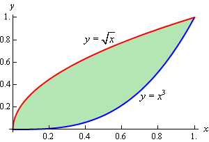
So, from the sketch we can see that that two inequalities are,
\[0 \le x \le 1\hspace{0.25in}{x^3} \le y \le \sqrt x \]We can now do the integral,
\[\begin{align*}\iint\limits_{D}{{4xy - {y^3}\,dA}} & = \int_{{\,0}}^{{\,1}}{{\int_{{\,{x^3}}}^{{\,\sqrt x }}{{4xy - {y^3}\,dy}}\,dx}}\\ & = \int_{{\,0}}^{{\,1}}{{\left. {\left( {2x{y^2} - \frac{1}{4}{y^4}} \right)} \right|_{{x^3}}^{\sqrt x }\,dx}}\\ & = \int_{{\,0}}^{{\,1}}{{\frac{7}{4}{x^2} - 2{x^7} + \frac{1}{4}{x^{12}}\,dx}}\\ & = \left. {\left( {\frac{7}{{12}}{x^3} - \frac{1}{4}{x^8} + \frac{1}{{52}}{x^{13}}} \right)} \right|_0^1 = \frac{{55}}{{156}}\end{align*}\]c \(\displaystyle \iint\limits_{D}{{6{x^2} - 40y\,dA}}\), \(D\) is the triangle with vertices \(\left( {0,3} \right)\), \(\left( {1,1} \right)\), and \(\left( {5,3} \right)\). Show Solution
We got even less information about the region this time. Let’s start this off by sketching the triangle.
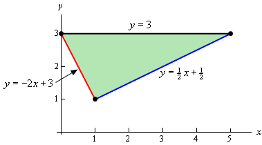
Since we have two points on each edge it is easy to get the equations for each edge and so we’ll leave it to you to verify the equations.
Now, there are two ways to describe this region. If we use functions of \(x\), as shown in the image we will have to break the region up into two different pieces since the lower function is different depending upon the value of \(x\). In this case the region would be given by \(D = {D_1} \cup {D_2}\) where,
\[\begin{align*}{D_1} & = \left\{ {\left( {x,y} \right)|0 \le x \le 1,\,\,\, - 2x + 3 \le y \le 3} \right\}\\ {D_2} & = \left\{ {\left( {x,y} \right)|1 \le x \le 5,\,\,\,\frac{1}{2}x + \frac{1}{2} \le y \le 3} \right\}\end{align*}\]Note the \( \cup \) is the “union” symbol and just means that \(D\) is the region we get by combing the two regions. If we do this then we’ll need to do two separate integrals, one for each of the regions.
To avoid this we could turn things around and solve the two equations for \(x\) to get,
\[\begin{align*}y & = - 2x + 3\hspace{0.5in} \Rightarrow \hspace{0.5in}x = - \frac{1}{2}y + \frac{3}{2}\\ y & = \frac{1}{2}x + \frac{1}{2}\hspace{0.5in} \Rightarrow \hspace{0.5in}x = 2y - 1\end{align*}\]If we do this we can notice that the same function is always on the right and the same function is always on the left and so the region is,
\[D = \left\{ {\left( {x,y} \right)|\,\, - \frac{1}{2}y + \frac{3}{2} \le x \le 2y - 1,\,\,\,1 \le y \le 3} \right\}\]Writing the region in this form means doing a single integral instead of the two integrals we’d have to do otherwise.
Either way should give the same answer and so we can get an example in the notes of splitting a region up let’s do both integrals.
Solution 1
\[\begin{align*}\iint\limits_{D}{{6{x^2} - 40y\,dA}} & = \iint\limits_{{{D_1}}}{{6{x^2} - 40y\,dA}} + \iint\limits_{{{D_2}}}{{6{x^2} - 40y\,dA}}\\ & = \int_{{\,0}}^{{\,1}}{{\int_{{\, - 2x + 3}}^{{\,3}}{{6{x^2} - 40y\,dy}}\,dx}} + \int_{{\,1}}^{{\,5}}{{\int_{{\,\frac{1}{2}x + \frac{1}{2}}}^{{\,3}}{{6{x^2} - 40y\,dy}}\,dx}}\\ & = \int_{{\,0}}^{{\,1}}{{\left. {\left( {6{x^2}y - 20{y^2}} \right)} \right|_{ - 2x + 3}^3\,dx}} + \int_{{\,1}}^{{\,5}}{{\left. {\left( {6{x^2}y - 20{y^2}} \right)} \right|_{\frac{1}{2}x + \frac{1}{2}}^3\,dx}}\\ & = \int_{{\,0}}^{{\,1}}{{12{x^3} - 180 + 20{{\left( {3 - 2x} \right)}^2}\,dx}} + \int_{{\,1}}^{{\,5}}{{ - 3{x^3} + 15{x^2} - 180 + 20{{\left( {\frac{1}{2}x + \frac{1}{2}} \right)}^2}\,dx}}\\ & = \left. {\left( {3{x^4} - 180x - \frac{{10}}{3}{{\left( {3 - 2x} \right)}^3}} \right)} \right|_0^1 + \left. {\left( { - \frac{3}{4}{x^4} + 5{x^3} - 180x + \frac{{40}}{3}{{\left( {\frac{1}{2}x + \frac{1}{2}} \right)}^3}} \right)} \right|_1^5\\ & = - \frac{{935}}{3}\end{align*}\]That was a lot of work. Notice however, that after we did the first substitution that we didn’t multiply everything out. The two quadratic terms can be easily integrated with a basic Calc I substitution and so we didn’t bother to multiply them out. We’ll do that on occasion to make some of these integrals a little easier.
Solution 2
This solution will be a lot less work since we are only going to do a single integral.
So, the numbers were a little messier, but other than that there was much less work for the same result. Also notice that again we didn’t cube out the two terms as they are easier to deal with using a Calc I substitution.
As the last part of the previous example has shown us we can integrate these integrals in either order (i.e. \(x\) followed by \(y\) or \(y\) followed by \(x\)), although often one order will be easier than the other. In fact, there will be times when it will not even be possible to do the integral in one order while it will be possible to do the integral in the other order.
Also, do not forget about Calculus I substitutions. Students often just get in a hurry and multiply everything out after doing the integral evaluation and end up missing a really simple Calculus I substitution that avoids the hassle of multiplying everything out. Calculus I substitutions don’t always show up, but when they do they almost always simplify the work for the rest of the problem.
Let’s see a couple of examples of these kinds of integrals.
- \(\displaystyle \int_{{\,0}}^{{\,3}}{{\int_{{\,{x^2}}}^{{\,9}}{{{x^3}{{\bf{e}}^{{y^3}}}\,dy}}\,dx}}\)
- \(\displaystyle \int_{{\,0}}^{{\,8}}{{\int_{{\,\sqrt[3]{y}}}^{{\,2}}{{\sqrt {{x^4} + 1} \,dx}}\,dy}}\)
First, notice that if we try to integrate with respect to \(y\) we can’t do the integral because we would need a \({y^2}\) in front of the exponential in order to do the \(y\) integration. We are going to hope that if we reverse the order of integration we will get an integral that we can do.
Now, when we say that we’re going to reverse the order of integration this means that we want to integrate with respect to \(x\) first and then \(y\). Note as well that we can’t just interchange the integrals, keeping the original limits, and be done with it. This would not fix our original problem and in order to integrate with respect to \(x\) we can’t have \(x\)’s in the limits of the integrals. Even if we ignored that the answer would not be a constant as it should be.
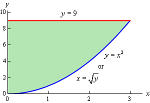
So, let’s see how we reverse the order of integration. The best way to reverse the order of integration is to first sketch the region given by the original limits of integration. From the integral we see that the inequalities that define this region are,
\[\begin{array}{c}0 \le x \le 3\\ {x^2} \le y \le 9\end{array}\]These inequalities tell us that we want the region with \(y = {x^2}\) on the lower boundary and \(y = 9\) on the upper boundary that lies between \(x = 0\) and \(x = 3\). Here is a sketch of that region.
Since we want to integrate with respect to \(x\) first we will need to determine limits of \(x\) (probably in terms of \(y\)) and then get the limits on the \(y\)’s. Here they are for this region.
\[\begin{array}{c}0 \le x \le \sqrt y \\ 0 \le y \le 9\end{array}\]Any horizontal line drawn in this region will start at \(x = 0\) and end at \(x = \sqrt y \) and so these are the limits on the \(x\)’s and the range of \(y\)’s for the regions is 0 to 9.
The integral, with the order reversed, is now,
\[\int_{{\,0}}^{{\,3}}{{\int_{{\,{x^2}}}^{{\,9}}{{{x^3}{{\bf{e}}^{{y^3}}}\,dy}}\,dx}} = \int_{{\,0}}^{{\,9}}{{\int_{{\,0}}^{{\,\sqrt y }}{{{x^3}{{\bf{e}}^{{y^3}}}\,dx}}\,dy}}\]and notice that we can do the first integration with this order. We’ll also hope that this will give us a second integral that we can do. Here is the work for this integral.
\[\begin{align*}\int_{{\,0}}^{{\,3}}{{\int_{{\,{x^2}}}^{{\,9}}{{{x^3}{{\bf{e}}^{{y^3}}}\,dy}}\,dx}} & = \int_{{\,0}}^{{\,9}}{{\int_{{\,0}}^{{\,\sqrt y }}{{{x^3}{{\bf{e}}^{{y^3}}}\,dx}}\,dy}}\\ & = \int_{{\,0}}^{{\,9}}{{\left. {\frac{1}{4}{x^4}{{\bf{e}}^{{y^3}}}} \right|_0^{\sqrt y }\,dy}}\\ & = \int_{{\,0}}^{{\,9}}{{\frac{1}{4}{y^2}{{\bf{e}}^{{y^3}}}\,dy}}\\ & = \left. {\frac{1}{{12}}{{\bf{e}}^{{y^3}}}} \right|_0^9\\ & = \frac{1}{{12}}\left( {{{\bf{e}}^{729}} - 1} \right)\end{align*}\]So, as we hoped, we were able to do the integral once we interchanged the order of integration.
b \(\displaystyle \int_{{\,0}}^{{\,8}}{{\int_{{\,\sqrt[3]{y}}}^{{\,2}}{{\sqrt {{x^4} + 1} \,dx}}\,dy}}\) Show Solution
As with the first integral we cannot do this integral by integrating with respect to \(x\) first so we’ll hope that by reversing the order of integration we will get something that we can integrate. Here are the limits for the variables that we get from this integral.
\[\begin{array}{c}\sqrt[3]{y} \le x \le 2\\ 0 \le y \le 8\end{array}\]and here is a sketch of this region.
![This is the 2D graph on the domain 0<x<2 of $y=x^{3}$. The right edge is marked as the line x=2. It is also noted that the curve could also be written as $x=\sqrt[3]{y}$. The area between the function and the x-axis has been shaded in.](DIGeneralRegion_Files/image006.png)
So, if we reverse the order of integration we get the following limits.
\[\begin{array}{c}0 \le x \le 2\\ 0 \le y \le {x^3}\end{array}\]The integral is then,
\[\begin{align*}\int_{{\,0}}^{{\,8}}{{\int_{{\,\sqrt[3]{y}}}^{{\,2}}{{\sqrt {{x^4} + 1} \,dx}}\,dy}} & = \int_{{\,0}}^{{\,2}}{{\int_{{\,0}}^{{\,{x^3}}}{{\sqrt {{x^4} + 1} \,dy}}\,dx}}\\ & = \int_{{\,0}}^{{\,2}}{{\left. {y\sqrt {{x^4} + 1} } \right|_0^{{x^3}}\,dx}}\\ & = \int_{{\,0}}^{{\,2}}{{{x^3}\sqrt {{x^4} + 1} \,dx}} = \frac{1}{6}\left( {{{17}^{\frac{3}{2}}} - 1} \right)\end{align*}\]The final topic of this section is two geometric interpretations of a double integral. The first interpretation is an extension of the idea that we used to develop the idea of a double integral in the first section of this chapter. We did this by looking at the volume of the solid that was below the surface of the function \(z = f\left( {x,y} \right)\) and over the rectangle \(R\) in the \(xy\)-plane. This idea can be extended to more general regions.
The volume of the solid that lies below the surface given by \(z = f\left( {x,y} \right)\) and above the region \(D\) in the \(xy\)-plane is given by,
\[V = \iint\limits_{D}{{f\left( {x,y} \right)\,dA}}\]Here is the graph of the surface and we’ve tried to show the region in the \(xy\)-plane below the surface.
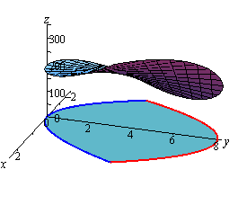
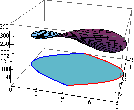
Here is a sketch of the region in the \(xy\)-plane by itself.
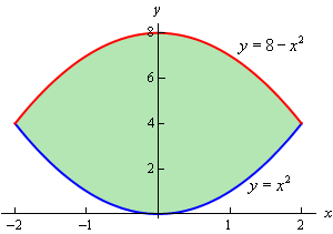
By setting the two bounding equations equal we can see that they will intersect at \(x = 2\) and \(x = - 2\). So, the inequalities that will define the region \(D\) in the \(xy\)-plane are,
\[\begin{array}{c} - 2 \le x \le 2\\ {x^2} \le y \le 8 - {x^2}\end{array}\]The volume is then given by,
\[\begin{align*}V &= \iint\limits_{D}{{16xy + 200\,dA}}\\ & = \int_{{ - 2}}^{{\,2}}{{\int_{{{x^2}}}^{{8 - {x^2}}}{{16xy + 200\,dy}}\,dx}}\\ & = \int_{{ - 2}}^{{\,2}}{{\left. {\left( {8x{y^2} + 200y} \right)} \right|_{{x^2}}^{8 - {x^2}}\,dx}}\\ & = \int_{{ - 2}}^{{\,2}}{{ - 128{x^3} - 400{x^2} + 512x + 1600\,dx}}\\ & = \left. {\left( { - 32{x^4} - \frac{{400}}{3}{x^3} + 256{x^2} + 1600x} \right)} \right|_{ - 2}^2 = \frac{{12800}}{3}\end{align*}\]This example is a little different from the previous one. Here the region \(D\) is not explicitly given so we’re going to have to find it. First, notice that the last two planes are really telling us that we won’t go past the \(xy\)-plane and the \(yz\)-plane when we reach them.
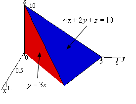
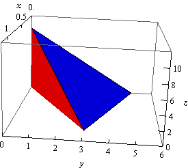
The first plane, \(4x + 2y + z = 10\), is the top of the volume and so we are really looking for the volume under,
\[z = 10 - 4x - 2y\]and above the region \(D\) in the \(xy\)-plane. The second plane, \(y = 3x\) (yes that is a plane), gives one of the sides of the volume as shown below.
The region \(D\) will be the region in the \(xy\)-plane (i.e. \(z = 0\)) that is bounded by \(y = 3x\), \(x = 0\), and the line where \(z + 4x + 2y = 10\) intersects the \(xy\)-plane. We can determine where \(z + 4x + 2y = 10\) intersects the \(xy\)-plane by plugging \(z = 0\) into it.
\[0 + 4x + 2y = 10\hspace{0.25in} \Rightarrow \hspace{0.25in}2x + y = 5\hspace{0.25in} \Rightarrow \hspace{0.25in}y = - 2x + 5\]So, here is a sketch the region \(D\).
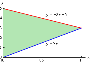
The region \(D\) is really where this solid will sit on the \(xy\)-plane and here are the inequalities that define the region.
\[\begin{array}{c}0 \le x \le 1\\ 3x \le y \le - 2x + 5\end{array}\]Here is the volume of this solid.
\[\begin{align*}V & = \iint\limits_{D}{{10 - 4x - 2y\,dA}}\\ & = \int_{0}^{{\,1}}{{\int_{{3x}}^{{ - 2x + 5}}{{10 - 4x - 2y\,dy}}\,dx}}\\ & = \int_{0}^{{\,1}}{{\left. {\left( {10y - 4xy - {y^2}} \right)} \right|_{3x}^{ - 2x + 5}\,dx}}\\ & = \int_{0}^{{\,1}}{{25{x^2} - 50x + 25\,dx}}\\ & = \left. {\left( {\frac{{25}}{3}{x^3} - 25{x^2} + 25x} \right)} \right|_0^1 = \frac{{25}}{3}\end{align*}\]Note that more generally,
\[V = \iint\limits_{D}{{f\left( {x,y} \right)\,dA}}\]gives the net volume between the graph of \(z = f\left( {x,y} \right)\) and the region \(D\) in the \(xy\)-plane. Regions that are below the \(xy\)-plane have a negative volume and regions that are above the \(xy\)-plane have a positive volume.
We saw a similar idea in Calculus I where,
\[A = \int_{a}^{b}{{f\left( x \right)\,dx}}\]gives the net area between the curve given by \(y = f\left( x \right)\) and the \(x\)-axis on the interval \(\left[ {a,b} \right]\).
The second geometric interpretation of a double integral is the following.
This is easy to see why this is true in general. Let’s suppose that we want to find the area of the region shown below.
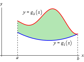
From Calculus I we know that this area can be found by the integral,
\[A = \int_{{\,a}}^{{\,b}}{{{g_2}\left( x \right) - {g_1}\left( x \right)\,dx}}\]Or in terms of a double integral we have,
\[\begin{align*}{\mbox{Area of }}D & = \iint\limits_{D}{{dA}}\\ & = \int_{{\,a}}^{{\,b}}{{\int_{{\,{g_1}\left( x \right)}}^{{\,{g_2}\left( x \right)}}{{dy}}\,dx}}\\ & = \int_{{\,a}}^{{\,b}}{{\left. y \right|_{{g_1}\left( x \right)}^{{g_2}\left( x \right)}\,dx}} = \int_{{\,a}}^{{\,b}}{{{g_2}\left( x \right) - {g_1}\left( x \right)\,dx}}\end{align*}\]This is exactly the same formula we had in Calculus I.