Calculus I - Minimum and Maximum Values

Show Mobile Notice Show All Notes Hide All Notes

Mobile Notice

You appear to be on a device with a "narrow" screen width (i.e. you are probably on a mobile phone). Due to the nature of the mathematics on this site it is best views in landscape mode. If your device is not in landscape mode many of the equations will run off the side of your device (should be able to scroll to see them) and some of the menu items will be cut off due to the narrow screen width.

Section 4.3 : Minimum and Maximum Values

Many of our applications in this chapter will revolve around minimum and maximum values of a function. While we can all visualize the minimum and maximum values of a function we want to be a little more specific in our work here. In particular, we want to differentiate between two types of minimum or maximum values. The following definition gives the types of minimums and/or maximums values that we’ll be looking at.

Definition

We say that $f\left( x \right)$ has an absolute (or global) maximum at $x = c$ if$f\left( x \right) \le f\left( c \right)$ for every $x$ in the domain we are working on.
We say that $f\left( x \right)$ has a relative (or local) maximum at $x = c$ if $f\left( x \right) \le f\left( c \right)$ for every $x$ in some open interval around $x = c$.
We say that $f\left( x \right)$ has an absolute (or global) minimum at $x = c$ if $f\left( x \right) \ge f\left( c \right)$ for every $x$ in the domain we are working on.
We say that $f\left( x \right)$ has a relative (or local) minimum at $x = c$ if$f\left( x \right) \ge f\left( c \right)$ for every $x$ in some open interval around $x = c$.

Note that when we say an “open interval around$x = c$” we mean that we can find some interval $\left( {a,b} \right)$, not including the endpoints, such that $a < c < b$. Or, in other words, $c$ will be contained somewhere inside the interval and will not be either of the endpoints.

Also, we will collectively call the minimum and maximum points of a function the extrema of the function. So, relative extrema will refer to the relative minimums and maximums while absolute extrema refer to the absolute minimums and maximums.

Now, let’s talk a little bit about the subtle difference between the absolute and relative in the definition above.

We will have an absolute maximum (or minimum) at $x = c$ provided $f\left( c \right)$ is the largest (or smallest) value that the function will ever take on the domain that we are working on. Also, when we say the “domain we are working on” this simply means the range of $x$’s that we have chosen to work with for a given problem. There may be other values of $x$ that we can actually plug into the function but have excluded them for some reason.

A relative maximum or minimum is slightly different. All that’s required for a point to be a relative maximum or minimum is for that point to be a maximum or minimum in some interval of $x$’s around $x = c$. There may be larger or smaller values of the function at some other place, but relative to $x = c$, or local to $x = c$, $f\left( c \right)$ is larger or smaller than all the other function values that are near it.

Note as well that in order for a point to be a relative extrema we must be able to look at function values on both sides of $x = c$ to see if it really is a maximum or minimum at that point. This means that relative extrema do not occur at the end points of a domain. They can only occur interior to the domain.

There is actually some debate on the preceding point. Some folks do feel that relative extrema can occur on the end points of a domain. However, in this class we will be using the definition that says that they can’t occur at the end points of a domain. This will be discussed in a little more detail at the end of the section once we have a relevant fact taken care of.

It’s usually easier to get a feel for the definitions by taking a quick look at a graph.

This is a sketch of some unknown function. The left most point is in the third quadrant and marked as “a” is the lowest point on the graph. From here the graph increases up into the third quadrant to a point label as “b” and marked as “Rel. Max.” At this point the graph reaches a peak but is not the highest point on the graph. The graph now decreases back into the third quadrant to a point labeled as “c” and marked as “Rel. Min.”. At this point the graph reaches a valley but is not the lowest point on the graph. The graph now increases up into the first quadrant to a point labeled as “d” and marked as “Abs. & Rel. Max.”. At this point the graph reaches a peak and is the highest point on the graph. The graph then decreases into the fourth quadrant and ends as a point labeled as “e”.

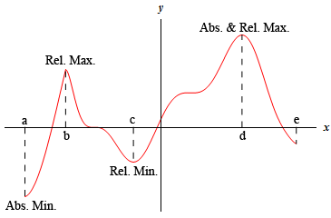
For the function shown in this graph we have relative maximums at $x = b$ and $x = d$. Both of these points are relative maximums since they are interior to the domain shown and are the largest point on the graph in some interval around the point. We also have a relative minimum at $x = c$ since this point is interior to the domain and is the lowest point on the graph in an interval around it. The far-right end point, $x = e$, will not be a relative minimum since it is an end point.

The function will have an absolute maximum at $x = d$ and an absolute minimum at $x = a$. These two points are the largest and smallest that the function will ever be. We can also notice that the absolute extrema for a function will occur at either the endpoints of the domain or at relative extrema. We will use this idea in later sections so it’s more important than it might seem at the present time.

Let’s take a quick look at some examples to make sure that we have the definitions of absolute extrema and relative extrema straight.

Example 1 Identify the absolute extrema and relative extrema for the following function. \[f\left( x \right) = {x^2}\hspace{0.25in}{\mbox{on}}\hspace{0.25in}\left[ { - 1,2} \right]\]

Show Solution

Since this function is easy enough to graph let’s do that. However, we only want the graph on the interval $\left[ { - 1,2} \right]$. Here is the graph,

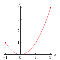
$Graph of $f\left( x \right)={{x}^{2}}$ on the domain $-1 \le x \le 2$ with dots at the (-1,1) and (2,4) to indicate that the graph does not extend past these two points.$

Note that we used dots at the end of the graph to remind us that the graph ends at these points.

We can now identify the extrema from the graph. It looks like we’ve got a relative and absolute minimum of zero at $x = 0$ and an absolute maximum of four at $x = 2$. Note that $x = - 1$ is not a relative maximum since it is at the end point of the interval.

This function doesn’t have any relative maximums.

As we saw in the previous example functions do not have to have relative extrema. It is completely possible for a function to not have a relative maximum and/or a relative minimum.

Example 2 Identify the absolute extrema and relative extrema for the following function. \[f\left( x \right) = {x^2}\hspace{0.25in}{\mbox{on}}\hspace{0.25in}\left[ { - 2,2} \right]\]

Show Solution

Here is the graph for this function.

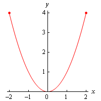
$Graph of $f\left( x \right)={{x}^{2}}$ on the domain $-2 \le x \le 2$ with dots at the (-2,4) and (2,4) to indicate that the graph does not extend past these two points.$

In this case we still have a relative and absolute minimum of zero at $x = 0$. We also still have an absolute maximum of four. However, unlike the first example this will occur at two points, $x = - 2$ and $x = 2$.

Again, the function doesn’t have any relative maximums.

As this example has shown there can only be a single absolute maximum or absolute minimum value, but they can occur at more than one place in the domain.

Example 3 Identify the absolute extrema and relative extrema for the following function. \[f\left( x \right) = {x^2}\]

Show Solution

In this case we’ve given no domain and so the assumption is that we will take the largest possible domain. For this function that means all the real numbers. Here is the graph.

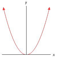
$Graph of $f\left( x \right)={{x}^{2}}$ with no domain specified and arrows at the ends pointing upwards to indicate the graph continues.$

In this case the graph doesn’t stop increasing at either end and so there are no maximums of any kind for this function. No matter which point we pick on the graph there will be points both larger and smaller than it on either side so we can’t have any maximums (of any kind, relative or absolute) in a graph.

We still have a relative and absolute minimum value of zero at $x = 0$.

So, some graphs can have minimums but not maximums. Likewise, a graph could have maximums but not minimums.

Example 4 Identify the absolute extrema and relative extrema for the following function. \[f\left( x \right) = {x^3}\hspace{0.25in}{\mbox{on}}\hspace{0.25in}\left[ { - 2,2} \right]\]

Show Solution

Here is the graph for this function.

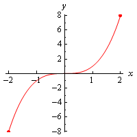
$Graph of $f\left( x \right)={{x}^{3}}$ on the domain $-2 \le x \le 2$ with dots at the (-2,-8) and (2,8) to indicate that the graph does not extend past these two points.$

This function has an absolute maximum of eight at $x = 2$ and an absolute minimum of negative eight at $x = - 2$. This function has no relative extrema.

So, a function doesn’t have to have relative extrema as this example has shown.

Example 5 Identify the absolute extrema and relative extrema for the following function. \[f\left( x \right) = {x^3}\]

Show Solution

Again, we aren’t restricting the domain this time so here’s the graph.

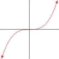
$Graph of $f\left( x \right)={{x}^{3}}$ with no domain specified and arrows at the ends to indicate the graph continues.$

In this case the function has no relative extrema and no absolute extrema.

As we’ve seen in the previous example functions don’t have to have any kind of extrema, relative or absolute.

Example 6 Identify the absolute extrema and relative extrema for the following function. \[f\left( x \right) = \cos \left( x \right)\]

Show Solution

We’ve not restricted the domain for this function. Here is the graph.

$Graph of $f\left( x \right)=\cos \left( x \right)$ on the domain $\left[ -3\pi ,3\pi \right]$ and arrows at the ends to indicate the graph continues.$

Cosine has extrema (relative and absolute) that occur at many points. Cosine has both relative and absolute maximums of 1 at

\[x = \ldots - 4\pi ,\, - 2\pi ,\,\,0,\,\,2\pi ,\,\,4\pi , \ldots \]

Cosine also has both relative and absolute minimums of -1 at

\[x = \ldots - 3\pi ,\, - \pi ,\,\,\pi ,\,\,3\pi , \ldots \]

As this example has shown a graph can in fact have extrema occurring at a large number (infinite in this case) of points.

We’ve now worked quite a few examples and we can use these examples to see a nice fact about absolute extrema. First let’s notice that all the functions above were continuous functions. Next notice that every time we restricted the domain to a closed interval (i.e. the interval contains its end points) we got absolute maximums and absolute minimums. Finally, in only one of the three examples in which we did not restrict the domain did we get both an absolute maximum and an absolute minimum.

These observations lead us the following theorem.

Extreme Value Theorem

Suppose that $f\left( x \right)$ is continuous on the interval $\left[ {a,b} \right]$ then there are two numbers $a \le c,d \le b$ so that $f\left( c \right)$ is an absolute maximum for the function and $f\left( d \right)$ is an absolute minimum for the function.

So, if we have a continuous function on an interval $\left[ {a,b} \right]$ then we are guaranteed to have both an absolute maximum and an absolute minimum for the function somewhere in the interval. The theorem doesn’t tell us where they will occur or if they will occur more than once, but at least it tells us that they do exist somewhere. Sometimes, all that we need to know is that they do exist.

This theorem doesn’t say anything about absolute extrema if we aren’t working on an interval. We saw examples of functions above that had both absolute extrema, one absolute extrema, and no absolute extrema when we didn’t restrict ourselves down to an interval.

The requirement that a function be continuous is also required in order for us to use the theorem. Consider the case of

\[f\left( x \right) = \frac{1}{{{x^2}}}\hspace{0.25in}{\mbox{on}}\hspace{0.25in}[ - 1,1]\]

Here’s the graph.

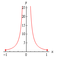
$Graph of $f\left( x \right)=\frac{1}{{{x}^{2}}}$ on the domain $-1 \le x \le 1$ with dots at the (-1,1) and (1,1) to indicate that the graph does not extend past these two points. There is also a gap as the graph approaches the y-axis to indicate that the graph will continue to move up the y-axis as it approaches.$

This function is not continuous at $x = 0$ as we move in towards zero the function is approaching infinity. So, the function does not have an absolute maximum. Note that it does have an absolute minimum however. In fact the absolute minimum occurs twice at both $x = - 1$ and $x = 1$.

If we changed the interval a little to say,

\[f\left( x \right) = \frac{1}{{{x^2}}}\hspace{0.25in}{\mbox{on}}\hspace{0.25in}\left[ {\frac{1}{2},1} \right]\]

the function would now have both absolute extrema. We may only run into problems if the interval contains the point of discontinuity. If it doesn’t then the theorem will hold.

We should also point out that just because a function is not continuous at a point that doesn’t mean that it won’t have both absolute extrema in an interval that contains that point. Below is the graph of a function that is not continuous at a point in the given interval and yet has both absolute extrema.

This is the graph of some unknown function. The left most point is in the third quadrant and labeled “a”. The graph increases to a peak (but not the highest point on the graph) in the second quadrant and then decreases into the third quadrant, passing through the y-axis into the fourth quadrant to a point labeled “c” that is the lowest point on the graph that is marked as the “Abs. Min.”. At this point the graph jumps up to a higher point that is still in the fourth quadrant and still at the same x value. The graph increases into the first quadrant to a peak (not highest point), decreases back into the fourth quadrant to a valley (not lowest point) and finally increases back into the first quadrant to the right most point that is labeled as “b” that is the highest point on the graph and marked as the “Abs. Max.”.

This graph is not continuous at $x = c$, yet it does have both an absolute maximum ($x = b$) and an absolute minimum ($x = c$). Also note that, in this case one of the absolute extrema occurred at the point of discontinuity, but it doesn’t need to. The absolute minimum could just have easily been at the other end point or at some other point interior to the region. The point here is that this graph is not continuous and yet does have both absolute extrema

The point of all this is that we need to be careful to only use the Extreme Value Theorem when the conditions of the theorem are met and not misinterpret the results if the conditions aren’t met.

In order to use the Extreme Value Theorem we must have an interval that includes its endpoints, often called a closed interval, and the function must be continuous on that interval. If we don’t have a closed interval and/or the function isn’t continuous on the interval then the function may or may not have absolute extrema.

We need to discuss one final topic in this section before moving on to the first major application of the derivative that we’re going to be looking at in this chapter.

Fermat’s Theorem

If $f\left( x \right)$ has a relative extrema at $x = c$ and $f'\left( c \right)$ exists then $x = c$ is a critical point of $f\left( x \right)$. In fact, it will be a critical point such that $f'\left( c \right) = 0$.

To see the proof of this theorem see the Proofs From Derivative Applications section of the Extras chapter.

Also note that we can say that $f'\left( c \right) = 0$ because we are also assuming that $f'\left( c \right)$ exists.

This theorem tells us that there is a nice relationship between relative extrema and critical points. In fact, it will allow us to get a list of all possible relative extrema. Since a relative extrema must be a critical point the list of all critical points will give us a list of all possible relative extrema.

Consider the case of $f\left( x \right) = {x^2}$. We saw that this function had a relative minimum at $x = 0$ in several earlier examples. So according to Fermat’s theorem $x = 0$ should be a critical point. The derivative of the function is,

\[f'\left( x \right) = 2x\]

Sure enough $x = 0$ is a critical point.

Be careful not to misuse this theorem. It doesn’t say that a critical point will be a relative extrema. To see this, consider the following case.

\[f\left( x \right) = {x^3}\hspace{0.25in}\hspace{0.25in}f'\left( x \right) = 3{x^2}\]

Clearly $x = 0$ is a critical point. However, we saw in an earlier example this function has no relative extrema of any kind. So, critical points do not have to be relative extrema.

Also note that this theorem says nothing about absolute extrema. An absolute extrema may or may not be a critical point.

Before we leave this section we need to discuss a couple of issues.

First, Fermat’s Theorem only works for critical points in which $f'\left( c \right) = 0$. This does not, however, mean that relative extrema won’t occur at critical points where the derivative does not exist. To see this consider $f\left( x \right) = \left| x \right|$. This function clearly has a relative minimum at $x = 0$ and yet in a previous section we showed in an example that $f'\left( 0 \right)$ does not exist.

What this all means is that if we want to locate relative extrema all we really need to do is look at the critical points as those are the places where relative extrema may exist.

Finally, recall that at that start of the section we stated that relative extrema will not exist at endpoints of the interval we are looking at. The reason for this is that if we allowed relative extrema to occur there it may well (and in fact most of the time) violate Fermat’s Theorem. There is no reason to expect end points of intervals to be critical points of any kind. Therefore, we do not allow relative extrema to exist at the endpoints of intervals.