Section 3.5 : Graphing Functions
Now we need to discuss graphing functions. If we recall from the previous section we said that \(f\left( x \right)\) is nothing more than a fancy way of writing \(y\). This means that we already know how to graph functions. We graph functions in exactly the same way that we graph equations. If we know ahead of time what the function is a graph of we can use that information to help us with the graph and if we don’t know what the function is ahead of time then all we need to do is plug in some \(x\)’s compute the value of the function (which is really a \(y\) value) and then plot the points.
Now, as we talked about when we first looked at graphing earlier in this chapter we’ll need to pick values of \(x\) to plug in and knowing the values to pick really only comes with experience. Therefore, don’t worry so much about the values of \(x\) that we’re using here. By the end of this chapter you’ll also be able to correctly pick these values.
Here are the function evaluations.
| \(x\) | \(f(x)\) | \(\left( {x,y} \right)\) |
|---|---|---|
| -1 | -7 | \(\left( { - 1, - 7} \right)\) |
| 0 | 0 | \(\left( {0,0} \right)\) |
| 1 | 1 | \(\left( {1,1} \right)\) |
| 2 | 2 | \(\left( {2,2} \right)\) |
| 3 | 9 | \(\left( {3,9} \right)\) |
Here is the sketch of the graph.
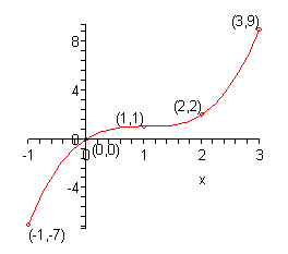
So, graphing functions is pretty much the same as graphing equations.
There is one function that we’ve seen to this point that we didn’t really see anything like when we were graphing equations in the first part of this chapter. That is piecewise functions. So, we should graph a couple of these to make sure that we can graph them as well.
Okay, now when we are graphing piecewise functions we are really graphing several functions at once, except we are only going to graph them on very specific intervals. In this case we will be graphing the following two functions,
\[\begin{align*} - {x^2} + 4\hspace{0.25in} & {\mbox{on}}\hspace{0.25in}x < 1\\ 2x - 1\hspace{0.25in} & {\mbox{on}}\hspace{0.25in}x \ge 1\end{align*}\]We’ll need to be a little careful with what is going on right at \(x = 1\) since technically that will only be valid for the bottom function. However, we’ll deal with that at the very end when we actually do the graph. For now, we will use \(x = 1\) in both functions.
The first thing to do here is to get a table of values for each function on the specified range and again we will use \(x = 1\) in both even though technically it only should be used with the bottom function.
| \(x\) | \( - {x^2} + 4\) | \(\left( {x,y} \right)\) |
|---|---|---|
| -2 | 0 | \(\left( { - 2,0} \right)\) |
| -1 | 3 | \(\left( { - 1,3} \right)\) |
| 0 | 4 | \(\left( {0,4} \right)\) |
| 1 | 3 | \(\left( {1,3} \right)\) |
| \(x\) | \(2x - 1\) | \(\left( {x,y} \right)\) |
|---|---|---|
| 1 | 1 | \(\left( {1,1} \right)\) |
| 2 | 3 | \(\left( {2,3} \right)\) |
| 3 | 5 | \(\left( {3,5} \right)\) |
Here is a sketch of the graph and notice how we denoted the points at \(x = 1\). For the top function we used an open dot for the point at \(x = 1\) and for the bottom function we used a closed dot at \(x = 1\). In this way we make it clear on the graph that only the bottom function really has a point at \(x = 1\).
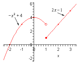
Notice that since the two graphs didn’t meet at \(x = 1\) we left a blank space in the graph. Do NOT connect these two points with a line. There really does need to be a break there to signify that the two portions do not meet at \(x = 1\).
Sometimes the two portions will meet at these points and at other times they won’t. We shouldn’t ever expect them to meet or not to meet until we’ve actually sketched the graph.
Let’s take a look at another example of a piecewise function.
In this case we will be graphing three functions on the ranges given above. So, as with the previous example we will get function values for each function in its specified range and we will include the endpoints of each range in each computation. When we graph we will acknowledge which function the endpoint actually belongs with by using a closed dot as we did previously. Also, the top and bottom functions are lines and so we don’t really need more than two points for these two. We’ll get a couple more points for the middle function.
| \(x\) | \(x + 3\) | \(\left( {x,y} \right)\) |
|---|---|---|
| -3 | 0 | \(\left( { - 3,0} \right)\) |
| -2 | 1 | \(\left( { - 2,1} \right)\) |
| \(x\) | \({x^2}\) | \(\left( {x,y} \right)\) |
|---|---|---|
| -2 | 4 | \(\left( { - 2,4} \right)\) |
| -1 | 1 | \(\left( { - 1,1} \right)\) |
| 0 | 0 | \(\left( {0,0} \right)\) |
| 1 | 1 | \(\left( {1,1} \right)\) |
| \(x\) | \( - x + 2\) | \(\left( {x,y} \right)\) |
|---|---|---|
| 1 | 1 | \(\left( {1,1} \right)\) |
| 2 | 0 | \(\left( {2,0} \right)\) |
Here is the sketch of the graph.
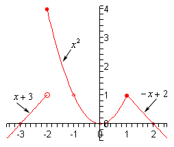
Note that in this case two of the portions met at the breaking point \(x = 1\) and at the other breaking point, \(x = - 2\), they didn’t meet up. As noted in the previous example sometimes they meet up and sometimes they won’t.