Section 13.1 : Limits
In this section we will take a look at limits involving functions of more than one variable. In fact, we will concentrate mostly on limits of functions of two variables, but the ideas can be extended out to functions with more than two variables.
Before getting into this let’s briefly recall how limits of functions of one variable work. We say that,
\[\mathop {\lim }\limits_{x \to a} f\left( x \right) = L\]provided,
\[\mathop {\lim }\limits_{x \to {a^ + }} f\left( x \right) = \mathop {\lim }\limits_{x \to {a^ - }} f\left( x \right) = L\]Also, recall that,
\[\mathop {\lim }\limits_{x \to {a^ + }} f\left( x \right)\]is a right hand limit and requires us to only look at values of \(x\) that are greater than \(a\). Likewise,
\[\mathop {\lim }\limits_{x \to {a^ - }} f\left( x \right)\]is a left hand limit and requires us to only look at values of \(x\) that are less than \(a\).
In other words, we will have \(\mathop {\lim }\limits_{x \to a} f\left( x \right) = L\) provided \(f\left( x \right)\) approaches \(L\) as we move in towards \(x = a\)(without letting \(x = a\)) from both sides.
Now, notice that in this case there are only two paths that we can take as we move in towards \(x = a\). We can either move in from the left or we can move in from the right. Then in order for the limit of a function of one variable to exist the function must be approaching the same value as we take each of these paths in towards \(x = a\).
With functions of two variables we will have to do something similar, except this time there is (potentially) going to be a lot more work involved. Let’s first address the notation and get a feel for just what we’re going to be asking for in these kinds of limits.
We will be asking to take the limit of the function \(f\left( {x,y} \right)\) as \(x\) approaches \(a\) and as \(y\) approaches \(b\). This can be written in several ways. Here are a couple of the more standard notations.
\[\mathop {\lim }\limits_{x \to a\atop y \to b} f\left( {x,y} \right)\hspace{0.5in}\mathop {\lim }\limits_{\left( {x,y} \right) \to \left( {a,b} \right)} f\left( {x,y} \right)\]We will use the second notation more often than not in this course. The second notation is also a little more helpful in illustrating what we are really doing here when we are taking a limit. In taking a limit of a function of two variables we are really asking what the value of \(f\left( {x,y} \right)\) is doing as we move the point \(\left( {x,y} \right)\) in closer and closer to the point \(\left( {a,b} \right)\) without actually letting it be \(\left( {a,b} \right)\).
Just like with limits of functions of one variable, in order for this limit to exist, the function must be approaching the same value regardless of the path that we take as we move in towards \(\left( {a,b} \right)\). The problem that we are immediately faced with is that there are literally an infinite number of paths that we can take as we move in towards \(\left( {a,b} \right)\). Here are a few examples of paths that we could take.
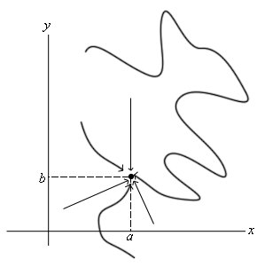
We put in a couple of straight line paths as well as a couple of “stranger” paths that aren’t straight line paths. Also, we only included 6 paths here and as you can see simply by varying the slope of the straight line paths there are an infinite number of these and then we would need to consider paths that aren’t straight line paths.
In other words, to show that a limit exists we would technically need to check an infinite number of paths and verify that the function is approaching the same value regardless of the path we are using to approach the point.
Luckily for us however we can use one of the main ideas from Calculus I limits to help us take limits here.
Definition
A function \(f\left( {x,y} \right)\) is continuous at the point \(\left( {a,b} \right)\) if,
\[\mathop {\lim }\limits_{\left( {x,y} \right) \to \left( {a,b} \right)} f\left( {x,y} \right) = f\left( {a,b} \right)\]From a graphical standpoint this definition means the same thing as it did when we first saw continuity in Calculus I. A function will be continuous at a point if the graph doesn’t have any holes or breaks at that point.
How can this help us take limits? Well, just as in Calculus I, if you know that a function is continuous at \(\left( {a,b} \right)\) then you also know that
\[\mathop {\lim }\limits_{\left( {x,y} \right) \to \left( {a,b} \right)} f\left( {x,y} \right) = f\left( {a,b} \right)\]must be true. So, if we know that a function is continuous at a point then all we need to do to take the limit of the function at that point is to plug the point into the function.
All the standard functions that we know to be continuous are still continuous even if we are plugging in more than one variable now. We just need to watch out for division by zero, square roots of negative numbers, logarithms of zero or negative numbers, etc.
Note that the idea about paths is one that we shouldn’t forget since it is a nice way to determine if a limit doesn’t exist. If we can find two paths upon which the function approaches different values as we get near the point then we will know that the limit doesn’t exist.
Let’s take a look at a couple of examples.
- \(\mathop {\lim }\limits_{\left( {x,y,z} \right) \to \left( {2,1, - 1} \right)} 3{x^2}z + yx\cos \left( {\pi x - \pi z} \right)\)
- \(\displaystyle \mathop {\lim }\limits_{\left( {x,y} \right) \to \left( {5,1} \right)} \frac{{xy}}{{x + y}}\)
Okay, in this case the function is continuous at the point in question and so all we need to do is plug in the values and we’re done.
\[\mathop {\lim }\limits_{\left( {x,y,z} \right) \to \left( {2,1, - 1} \right)} 3{x^2}z + yx\cos \left( {\pi x - \pi z} \right) = 3{\left( 2 \right)^2}\left( { - 1} \right) + \left( 1 \right)\left( 2 \right)\cos \left( {2\pi + \pi } \right) = - 14\]b \(\displaystyle \mathop {\lim }\limits_{\left( {x,y} \right) \to \left( {5,1} \right)} \frac{{xy}}{{x + y}}\) Show Solution
In this case the function will not be continuous along the line \(y = - x\) since we will get division by zero when this is true. However, for this problem that is not something that we will need to worry about since the point that we are taking the limit at isn’t on this line.
Therefore, all that we need to do is plug in the point since the function is continuous at this point.
\[\mathop {\lim }\limits_{\left( {x,y} \right) \to \left( {5,1} \right)} \frac{{xy}}{{x + y}} = \frac{5}{6}\]In the previous example there wasn’t really anything to the limits. The functions were continuous at the point in question and so all we had to do was plug in the point. That, of course, will not always be the case so let’s work a few examples that are more typical of those you’ll see here.
In this case the function is not continuous at the point in question (clearly division by zero). However, that does not mean that the limit can’t be done. We saw many examples of this in Calculus I where the function was not continuous at the point we were looking at and yet the limit did exist.
In the case of this limit notice that we can factor both the numerator and denominator of the function as follows,
\[\mathop {\lim }\limits_{\left( {x,y} \right) \to \left( {1,1} \right)} \frac{{2{x^2} - xy - {y^2}}}{{{x^2} - {y^2}}} = \mathop {\lim }\limits_{\left( {x,y} \right) \to \left( {1,1} \right)} \frac{{\left( {2x + y} \right)\left( {x - y} \right)}}{{\left( {x - y} \right)\left( {x + y} \right)}} = \mathop {\lim }\limits_{\left( {x,y} \right) \to \left( {1,1} \right)} \frac{{2x + y}}{{x + y}}\]So, just as we saw in many examples in Calculus I, upon factoring and canceling common factors we arrive at a function that in fact we can take the limit of. So, to finish out this example all we need to do is actually take the limit.
Taking the limit gives,
\[\mathop {\lim }\limits_{\left( {x,y} \right) \to \left( {1,1} \right)} \frac{{2{x^2} - xy - {y^2}}}{{{x^2} - {y^2}}} = \mathop {\lim }\limits_{\left( {x,y} \right) \to \left( {1,1} \right)} \frac{{2x + y}}{{x + y}} = \frac{3}{2}\]Before we move on to the next set of examples we should note that the situation in the previous example is what generally happened in many limit examples/problems in Calculus I. In Calculus III however, this tends to be the exception in the examples/problems as the next set of examples will show. In other words, do not expect most of these types of limits to just factor and then exist as they did in Calculus I.
- \(\displaystyle \mathop {\lim }\limits_{\left( {x,y} \right) \to \left( {0,0} \right)} \frac{{{x^2}{y^2}}}{{{x^4} + 3{y^4}}}\)
- \(\displaystyle \mathop {\lim }\limits_{\left( {x,y} \right) \to \left( {0,0} \right)} \frac{{{x^3}y}}{{{x^6} + {y^2}}}\)
In this case the function is not continuous at the point in question and so we can’t just plug in the point. Also, note that, unlike the previous example, we can’t factor this function and do some canceling so that the limit can be taken.
Therefore, since the function is not continuous at the point and because there is no factoring we can do, there is at least a chance that the limit doesn’t exist. If we could find two different paths to approach the point that gave different values for the limit then we would know that the limit didn’t exist. Two of the more common paths to check are the \(x\) and \(y\)-axis so let’s try those.
Before actually doing this we need to address just what exactly do we mean when we say that we are going to approach a point along a path. When we approach a point along a path we will do this by either fixing \(x\) or \(y\) or by relating \(x\) and \(y\) through some function. In this way we can reduce the limit to just a limit involving a single variable which we know how to do from Calculus I.
So, let’s see what happens along the \(x\)-axis. If we are going to approach \(\left( {0,0} \right)\) along the \(x\)-axis we can take advantage of the fact that that along the \(x\)-axis we know that \(y = 0\). This means that, along the \(x\)-axis, we will plug in \(y = 0\) into the function and then take the limit as \(x\) approaches zero.
\[\mathop {\lim }\limits_{\left( {x,y} \right) \to \left( {0,0} \right)} \frac{{{x^2}{y^2}}}{{{x^4} + 3{y^4}}} = \mathop {\lim }\limits_{\left( {x,0} \right) \to \left( {0,0} \right)} \frac{{{x^2}{{\left( 0 \right)}^2}}}{{{x^4} + 3{{\left( 0 \right)}^4}}} = \mathop {\lim }\limits_{\left( {x,0} \right) \to \left( {0,0} \right)} 0 = 0\]So, along the \(x\)-axis the function will approach zero as we move in towards the origin.
Now, let’s try the \(y\)-axis. Along this axis we have \(x = 0\) and so the limit becomes,
\[\mathop {\lim }\limits_{\left( {x,y} \right) \to \left( {0,0} \right)} \frac{{{x^2}{y^2}}}{{{x^4} + 3{y^4}}} = \mathop {\lim }\limits_{\left( {0,y} \right) \to \left( {0,0} \right)} \frac{{{{\left( 0 \right)}^2}{y^2}}}{{{{\left( 0 \right)}^4} + 3{y^4}}} = \mathop {\lim }\limits_{\left( {0,y} \right) \to \left( {0,0} \right)} 0 = 0\]So, the same limit along two paths. Don’t misread this. This does NOT say that the limit exists and has a value of zero. This only means that the limit happens to have the same value along two paths.
Let’s take a look at a third fairly common path to take a look at. In this case we’ll move in towards the origin along the path \(y = x\). This is what we meant previously about relating \(x\) and \(y\) through a function.
To do this we will replace all the \(y\)’s with \(x\)’s and then let \(x\) approach zero. Let’s take a look at this limit.
\[\mathop {\lim }\limits_{\left( {x,y} \right) \to \left( {0,0} \right)} \frac{{{x^2}{y^2}}}{{{x^4} + 3{y^4}}} = \mathop {\lim }\limits_{\left( {x,x} \right) \to \left( {0,0} \right)} \frac{{{x^2}{x^2}}}{{{x^4} + 3{x^4}}} = \mathop {\lim }\limits_{\left( {x,x} \right) \to \left( {0,0} \right)} \frac{{{x^4}}}{{4{x^4}}} = \mathop {\lim }\limits_{\left( {x,x} \right) \to \left( {0,0} \right)} \frac{1}{4} = \frac{1}{4}\]So, a different value from the previous two paths and this means that the limit can’t possibly exist.
Note that we can use this idea of moving in towards the origin along a line with the more general path \(y = mx\) if we need to.
b \(\displaystyle \mathop {\lim }\limits_{\left( {x,y} \right) \to \left( {0,0} \right)} \frac{{{x^3}y}}{{{x^6} + {y^2}}}\) Show Solution
Okay, with this last one we again have continuity problems at the origin and again there is no factoring we can do that will allow the limit to be taken. So, again let’s see if we can find a couple of paths that give different values of the limit.
First, we will use the path \(y = x\). Along this path we have,
\[\mathop {\lim }\limits_{\left( {x,y} \right) \to \left( {0,0} \right)} \frac{{{x^3}y}}{{{x^6} + {y^2}}} = \mathop {\lim }\limits_{\left( {x,x} \right) \to \left( {0,0} \right)} \frac{{{x^3}x}}{{{x^6} + {x^2}}} = \mathop {\lim }\limits_{\left( {x,x} \right) \to \left( {0,0} \right)} \frac{{{x^4}}}{{{x^6} + {x^2}}} = \mathop {\lim }\limits_{\left( {x,x} \right) \to \left( {0,0} \right)} \frac{{{x^2}}}{{{x^4} + 1}} = 0\]Now, let’s try the path \(y = {x^3}\). Along this path the limit becomes,
\[\mathop {\lim }\limits_{\left( {x,y} \right) \to \left( {0,0} \right)} \frac{{{x^3}y}}{{{x^6} + {y^2}}} = \mathop {\lim }\limits_{\left( {x,{x^3}} \right) \to \left( {0,0} \right)} \frac{{{x^3}{x^3}}}{{{x^6} + {{\left( {{x^3}} \right)}^2}}} = \mathop {\lim }\limits_{\left( {x,{x^3}} \right) \to \left( {0,0} \right)} \frac{{{x^6}}}{{2{x^6}}} = \mathop {\lim }\limits_{\left( {x,{x^3}} \right) \to \left( {0,0} \right)} \frac{1}{2} = \frac{1}{2}\]We now have two paths that give different values for the limit and so the limit doesn’t exist.
As this limit has shown us we can, and often need, to use paths other than lines like we did in the first part of this example.
So, as we’ve seen in the previous example limits are a little different here from those we saw in Calculus I. Limits in multiple variables can be quite difficult to evaluate and we’ve shown several examples where it took a little work just to show that the limit does not exist.