Section 10.6 : Integral Test
The last topic that we discussed in the previous section was the harmonic series. In that discussion we stated that the harmonic series was a divergent series. It is now time to prove that statement. This proof will also get us started on the way to our next test for convergence that we’ll be looking at.
So, we will be trying to prove that the harmonic series,
\[\sum\limits_{n = 1}^\infty {\frac{1}{n}} \]diverges.
We’ll start this off by looking at an apparently unrelated problem. Let’s start off by asking what the area under \(f\left( x \right) = \frac{1}{x}\) on the interval \(\left[ {1,\infty } \right)\). From the section on Improper Integrals we know that this is,
\[\int_{{\,1}}^{{\,\infty }}{{\frac{1}{x}\,dx}} = \infty \]and so we called this integral divergent (yes, that’s the same term we’re using here with series….).
So, just how does that help us to prove that the harmonic series diverges? Well, recall that we can always estimate the area by breaking up the interval into segments and then sketching in rectangles and using the sum of the area all of the rectangles as an estimate of the actual area. Let’s do that for this problem as well and see what we get.
We will break up the interval into subintervals of width 1 and we’ll take the function value at the left endpoint as the height of the rectangle. The image below shows the first few rectangles for this area.
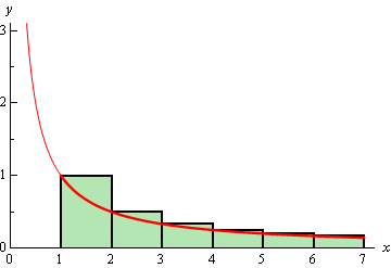
So, the area under the curve is approximately,
\[\begin{align*}A & \approx \left( {\frac{1}{1}} \right)\left( 1 \right) + \left( {\frac{1}{2}} \right)\left( 1 \right) + \left( {\frac{1}{3}} \right)\left( 1 \right) + \left( {\frac{1}{4}} \right)\left( 1 \right) + \left( {\frac{1}{5}} \right)\left( 1 \right) + \cdots \\ & = \frac{1}{1} + \frac{1}{2} + \frac{1}{3} + \frac{1}{4} + \frac{1}{5} + \cdots \\ & = \sum\limits_{n = 1}^\infty {\frac{1}{n}} \end{align*}\]Now note a couple of things about this approximation. First, each of the rectangles overestimates the actual area and secondly the formula for the area is exactly the harmonic series!
Putting these two facts together gives the following,
\[A \approx \sum\limits_{n = 1}^\infty {\frac{1}{n}} > \int_{{\,1}}^{{\,\infty }}{{\frac{1}{x}\,dx}} = \infty \]Notice that this tells us that we must have,
\[\sum\limits_{n = 1}^\infty {\frac{1}{n}} > \infty \hspace{0.5in} \Rightarrow \hspace{0.5in}\sum\limits_{n = 1}^\infty {\frac{1}{n}} = \infty \]Since we can’t really be larger than infinity the harmonic series must also be infinite in value. In other words, the harmonic series is in fact divergent.
So, we’ve managed to relate a series to an improper integral that we could compute and it turns out that the improper integral and the series have exactly the same convergence.
Let’s see if this will also be true for a series that converges. When discussing the Divergence Test we made the claim that
\[\sum\limits_{n = 1}^\infty {\frac{1}{{{n^2}}}} \]converges. Let’s see if we can do something similar to the above process to prove this.
We will try to relate this to the area under \(f\left( x \right) = \frac{1}{{{x^2}}}\) is on the interval \(\left[ {1,\infty } \right)\). Again, from the Improper Integral section we know that,
\[\int_{{\,1}}^{{\,\infty }}{{\frac{1}{{{x^2}}}\,dx}} = 1\]and so this integral converges.
We will once again try to estimate the area under this curve. We will do this in an almost identical manner as the previous part with the exception that instead of using the left end points for the height of our rectangles we will use the right end points. Here is a sketch of this case,
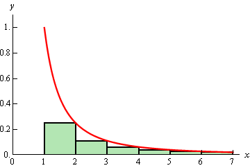
In this case the area estimation is,
\[\begin{align*}A & \approx \left( {\frac{1}{{{2^2}}}} \right)\left( 1 \right) + \left( {\frac{1}{{{3^2}}}} \right)\left( 1 \right) + \left( {\frac{1}{{{4^2}}}} \right)\left( 1 \right) + \left( {\frac{1}{{{5^2}}}} \right)\left( 1 \right) + \cdots \\ & = \frac{1}{{{2^2}}} + \frac{1}{{{3^2}}} + \frac{1}{{{4^2}}} + \frac{1}{{{5^2}}} + \cdots \end{align*}\]This time, unlike the first case, the area will be an underestimation of the actual area and the estimation is not quite the series that we are working with. Notice however that the only difference is that we’re missing the first term. This means we can do the following,
\[\sum\limits_{n = 1}^\infty {\frac{1}{{{n^2}}}} = \frac{1}{{{1^2}}} + \underbrace {\frac{1}{{{2^2}}} + \frac{1}{{{3^2}}} + \frac{1}{{{4^2}}} + \frac{1}{{{5^2}}} + \cdots }_{{\mbox{Area Estimation}}} < 1 + \int_{{\,1}}^{{\,\infty }}{{\frac{1}{{{x^2}}}\,dx}} = 1 + 1 = 2\]Or, putting all this together we see that,
\[\sum\limits_{n = 1}^\infty {\frac{1}{{{n^2}}}} < 2\]With the harmonic series this was all that we needed to say that the series was divergent. With this series however, this isn’t quite enough. For instance, \( - \infty < 2\), and if the series did have a value of \( - \infty \) then it would be divergent (when we want convergent). So, let’s do a little more work.
First, let’s notice that all the series terms are positive (that’s important) and that the partial sums are,
\[{s_n} = \sum\limits_{i = 1}^n {\frac{1}{{{i^2}}}} \]Because the terms are all positive we know that the partial sums must be an increasing sequence. In other words,
\[{s_n} = \sum\limits_{i = 1}^n {\frac{1}{{{i^2}}}} < \sum\limits_{i = 1}^{n + 1} {\frac{1}{{{i^2}}}} = {s_{n + 1}}\]In sn+1 we are adding a single positive term onto sn and so must get larger. Therefore, the partial sums form an increasing (and hence monotonic) sequence.
Also note that, since the terms are all positive, we can say,
\[{s_n} = \sum\limits_{i = 1}^n {\frac{1}{{{i^2}}}} < \sum\limits_{n = 1}^\infty {\frac{1}{{{n^2}}}} < 2\hspace{0.5in} \Rightarrow \hspace{0.25in}\,\,\,\,\,{s_n} < 2\]and so the sequence of partial sums is a bounded sequence.
In the second section on Sequences we gave a theorem that stated that a bounded and monotonic sequence was guaranteed to be convergent. This means that the sequence of partial sums is a convergent sequence. So, who cares right? Well recall that this means that the series must then also be convergent!
So, once again we were able to relate a series to an improper integral (that we could compute) and the series and the integral had the same convergence.
We went through a fair amount of work in both of these examples to determine the convergence of the two series. Luckily for us we don’t need to do all this work every time. The ideas in these two examples can be summarized in the following test.
Integral Test
Suppose that \(f\left( x \right)\) is a continuous, positive and decreasing function on the interval \(\left[ {k,\infty } \right)\) and that \(f\left( n \right) = {a_n}\) then,
- If \(\displaystyle \int_{{\,k}}^{{\,\infty }}{{f\left( x \right)\,dx}}\) is convergent so is \(\displaystyle \sum\limits_{\,n = k}^\infty {{a_n}} \).
- If \(\displaystyle \int_{{\,k}}^{{\,\infty }}{{f\left( x \right)\,dx}}\) is divergent so is \(\displaystyle \sum\limits_{\,n = k}^\infty {{a_n}} \).
A formal proof of this test can be found at the end of this section.
There are a couple of things to note about the integral test. First, the lower limit on the improper integral must be the same value that starts the series.
Second, the function does not actually need to be decreasing and positive everywhere in the interval. All that’s really required is that eventually the function is decreasing and positive. In other words, it is okay if the function (and hence series terms) increases or is negative for a while, but eventually the function (series terms) must decrease and be positive for all terms. To see why this is true let’s suppose that the series terms increase and or are negative in the range \(k \le n \le N\) and then decrease and are positive for \(n \ge N + 1\). In this case the series can be written as,
\[\sum\limits_{\,n = k}^\infty {{a_n}} = \sum\limits_{\,n = k}^N {{a_n}} + \sum\limits_{\,n = N + 1}^\infty {{a_n}} \]Now, the first series is nothing more than a finite sum (no matter how large \(N\) is) of finite terms and so will be finite. So, the original series will be convergent/divergent only if the second infinite series on the right is convergent/divergent and the test can be done on the second series as it satisfies the conditions of the test.
A similar argument can be made using the improper integral as well.
The requirement in the test that the function/series be decreasing and positive everywhere in the range is required for the proof. In practice however, we only need to make sure that the function/series is eventually a decreasing and positive function/series. Also note that when computing the integral in the test we don’t actually need to strip out the increasing/negative portion since the presence of a small range on which the function is increasing/negative will not change the integral from convergent to divergent or from divergent to convergent.
There is one more very important point that must be made about this test. This test does NOT give the value of a series. It will only give the convergence/divergence of the series. That’s it. No value. We can use the above series as a perfect example of this. All that the test gave us was that,
\[\sum\limits_{n = 1}^\infty {\frac{1}{{{n^2}}}} < 2\]So, we got an upper bound on the value of the series, but not an actual value for the series. In fact, from this point on we will not be asking for the value of a series we will only be asking whether a series converges or diverges. In a later section we look at estimating values of series, but even in that section still won’t actually be getting values of series.
Just for the sake of completeness the value of this series is known.
\[\sum\limits_{n = 1}^\infty {\frac{1}{{{n^2}}}} = \frac{{{\pi ^2}}}{6} = 1.644934... < 2\]Let’s work a couple of examples.
In this case the function we’ll use is,
\[f\left( x \right) = \frac{1}{{x\ln x}}\]This function is clearly positive and if we make \(x\) larger the denominator will get larger and so the function is also decreasing. Therefore, all we need to do is determine the convergence of the following integral.
\[\begin{align*}\int_{{\,2}}^{{\,\infty }}{{\frac{1}{{x\ln x}}\,dx}} & = \mathop {\lim }\limits_{t \to \infty } \int_{{\,2}}^{{\,t}}{{\frac{1}{{x\ln x}}\,dx}}\hspace{0.5in}u = \ln x\\ & = \mathop {\lim }\limits_{t \to \infty } \left. {\left( {\ln \left( {\ln x} \right)} \right)} \right|_2^t\\ & = \mathop {\lim }\limits_{t \to \infty } \left( {\ln \left( {\ln t} \right) - \ln \left( {\ln 2} \right)} \right)\\ & = \infty \end{align*}\]The integral is divergent and so the series is also divergent by the Integral Test.
The function that we’ll use in this example is,
\[f\left( x \right) = x{{\bf{e}}^{ - {x^2}}}\]This function is always positive on the interval that we’re looking at. Now we need to check that the function is decreasing. It is not clear that this function will always be decreasing on the interval given. We can use our Calculus I knowledge to help us however. The derivative of this function is,
\[f'\left( x \right) = {{\bf{e}}^{ - {x^2}}}\left( {1 - 2{x^2}} \right)\]This function has two critical points (which will tell us where the derivative changes sign) at \(x = \pm \frac{1}{{\sqrt 2 }}\). Since we are starting at \(n = 0\) we can ignore the negative critical point. Picking a couple of test points we can see that the function is increasing on the interval \(\left[ {0,\frac{1}{{\sqrt 2 }}} \right]\) and it is decreasing on \(\left[ {\frac{1}{{\sqrt 2 }},\infty } \right)\). Therefore, eventually the function will be decreasing and that’s all that’s required for us to use the Integral Test.
\[\begin{align*}\int_{{\,0}}^{{\,\infty }}{{x{{\bf{e}}^{ - {x^2}}}\,dx}} & = \mathop {\lim }\limits_{t \to \infty } \int_{{\,0}}^{{\,t}}{{x{{\bf{e}}^{ - {x^2}}}\,dx}}\hspace{0.5in}u = - {x^2}\\ & = \mathop {\lim }\limits_{t \to \infty } \left. {\left( { - \frac{1}{2}{{\bf{e}}^{ - {x^2}}}} \right)} \right|_0^t\\ & = \mathop {\lim }\limits_{t \to \infty } \left( {\frac{1}{2} - \frac{1}{2}{{\bf{e}}^{ - {t^2}}}} \right) = \frac{1}{2}\end{align*}\]The integral is convergent and so the series must also be convergent by the Integral Test.
We can use the Integral Test to get the following fact/test for some series.
Fact (The \(p\) –series Test)
If \(k > 0\) then \(\displaystyle \sum\limits_{n = k}^\infty {\frac{1}{{{n^p}}}} \) converges if \(p > 1\) and diverges if \(p \le 1\).
Sometimes the series in this fact are called \(p\)-series and so this fact is sometimes called the \(p\)-series test. This fact follows directly from the Integral Test and a similar fact we saw in the Improper Integral section. This fact says that the integral,
\[\int_{{\,k}}^{{\,\infty }}{{\frac{1}{{{x^p}}}\,dx}}\]converges if \(p > 1\) and diverges if \(p \le 1\).
Using the \(p\)-series test makes it very easy to determine the convergence of some series.
- \(\displaystyle \sum\limits_{n = 4}^\infty {\frac{1}{{{n^7}}}} \)
- \(\displaystyle \sum\limits_{n = 1}^\infty {\frac{1}{{\sqrt n }}} \)
In this case \(p = 7 > 1\) and so by this fact the series is convergent.
b \(\displaystyle \sum\limits_{n = 1}^\infty {\frac{1}{{\sqrt n }}} \) Show Solution
For this series \(p = \frac{1}{2} \le 1\) and so the series is divergent by the fact.
The last thing that we’ll do in this section is give a quick proof of the Integral Test. We’ve essentially done the proof already at the beginning of the section when we were introducing the Integral Test, but let’s go through it formally for a general function.
Proof of Integral Test
First, for the sake of the proof we’ll be working with the series \(\sum\limits_{\,n = 1}^\infty {{a_n}} \). The original test statement was for a series that started at a general \(n = k\) and while the proof can be done for that it will be easier if we assume that the series starts at \(n = 1\).
Another way of dealing with the \(n = k\) is we could do an index shift and start the series at \(n = 1\) and then do the Integral Test. Either way proving the test for \(n = 1\) will be sufficient.
Also note that while we allowed for the first few terms of the series to increase and/or be negative in working problems this proof does require that all the terms be decreasing and positive.
Let’s start off and estimate the area under the curve on the interval \(\left[ {1,n} \right]\) and we’ll underestimate the area by taking rectangles of width one and whose height is the right endpoint. This gives the following figure.
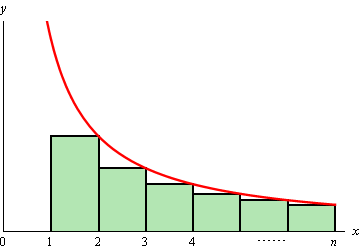
Now, note that,
\[f\left( 2 \right) = {a_2}\hspace{0.5in}f\left( 3 \right) = {a_3}\hspace{0.5in} \cdots \hspace{0.5in}f\left( n \right) = {a_n}\]
The approximate area is then,
\[A \approx \left( 1 \right)f\left( 2 \right) + \left( 1 \right)f\left( 3 \right) + \cdots + \left( 1 \right)f\left( n \right) = {a_2} + {a_3} + \cdots {a_n}\]
and we know that this underestimates the actual area so,
\[\sum\limits_{i = 2}^n {{a_i}} = {a_2} + {a_3} + \cdots {a_n} < \int_{{\,1}}^{{\,n}}{{f\left( x \right)\,dx}}\]
Now, let’s suppose that \(\int_{{\,1}}^{{\,\infty }}{{f\left( x \right)\,dx}}\) is convergent and so \(\int_{{\,1}}^{{\,\infty }}{{f\left( x \right)\,dx}}\) must have a finite value. Also, because \(f\left( x \right)\) is positive we know that,
\[\int_{{\,1}}^{{\,n}}{{f\left( x \right)\,dx}} < \int_{{\,1}}^{{\,\infty }}{{f\left( x \right)\,dx}}\]
This in turn means that,
\[\sum\limits_{i = 2}^n {{a_i}} < \int_{{\,1}}^{{\,n}}{{f\left( x \right)\,dx}} < \int_{{\,1}}^{{\,\infty }}{{f\left( x \right)\,dx}}\]
Our series starts at \(n = 1\) so this isn’t quite what we need. However, that’s easy enough to deal with.
\[\sum\limits_{i = 1}^n {{a_i}} = {a_1} + \sum\limits_{i = 2}^n {{a_i}} < {a_1} + \int_{{\,1}}^{{\,\infty }}{{f\left( x \right)\,dx}} = M\]
So, just what has this told us? Well we now know that the sequence of partial sums, \({s_n} = \sum\limits_{i = 1}^n {{a_i}} \) are bounded above by \(M\).
Next, because the terms are positive we also know that,
\[{s_n} \le {s_n} + {a_{n + 1}} = \sum\limits_{i = 1}^n {{a_i}} + {a_{n + 1}} = \sum\limits_{i = 1}^{n + 1} {{a_i}} = {s_{n + 1}}\hspace{0.25in} \Rightarrow \hspace{0.25in}{s_n} \le {s_{n + 1}}\]
and so the sequence \(\left\{ {{s_n}} \right\}_{n = 1}^\infty \) is also an increasing sequence. So, we now know that the sequence of partial sums \(\left\{ {{s_n}} \right\}_{n = 1}^\infty \) converges and hence our series \(\sum\limits_{n = 1}^\infty {{a_n}} \) is convergent.
So, the first part of the test is proven. The second part is somewhat easier. This time let’s overestimate the area under the curve by using the left endpoints of interval for the height of the rectangles as shown below.
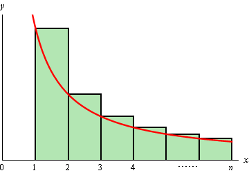
In this case the area is approximately,
\[A \approx \left( 1 \right)f\left( 1 \right) + \left( 1 \right)f\left( 2 \right) + \cdots + \left( 1 \right)f\left( {n - 1} \right) = {a_1} + {a_2} + \cdots {a_{n - 1}}\]
Since we know this overestimates the area we also then know that,
\[{s_{n - 1}} = \sum\limits_{i = 1}^{n - 1} {{a_i}} = {a_1} + {a_2} + \cdots {a_{n - 1}} > \int_{{\,1}}^{{\,n - 1}}{{f\left( x \right)\,dx}}\]
Now, suppose that \(\int_{{\,1}}^{{\,\infty }}{{f\left( x \right)\,dx}}\) is divergent. In this case this means that \(\int_{{\,1}}^{{\,n}}{{f\left( x \right)\,dx}} \to \infty \) as \(n \to \infty \) because \(f\left( x \right) \ge 0\). However, because \(n - 1 \to \infty \) as \(n \to \infty \) we also know that \(\int_{{\,1}}^{{\,n - 1}}{{f\left( x \right)\,dx}} \to \infty \).
Therefore, since \({s_{n - 1}} > \int_{{\,1}}^{{\,n - 1}}{{f\left( x \right)\,dx}}\) we know that as \(n \to \infty \) we must have \({s_{n - 1}} \to \infty \). This in turn tells us that \({s_n} \to \infty \) as \(n \to \infty \).
So, we now know that the sequence of partial sums, \(\left\{ {{s_n}} \right\}_{n = 1}^\infty \), is a divergent sequence and so \(\sum\limits_{n = 1}^\infty {{a_n}} \) is a divergent series.
It is important to note before leaving this section that in order to use the Integral Test the series terms MUST eventually be decreasing and positive. If they are not then the test doesn’t work. Also remember that the test only determines the convergence of a series and does NOT give the value of the series.