Section 12.5 : Functions of Several Variables
In this section we want to go over some of the basic ideas about functions of more than one variable.
First, remember that graphs of functions of two variables, \(z = f\left( {x,y} \right)\) are surfaces in three dimensional space. For example, here is the graph of \(z = 2{x^2} + 2{y^2} - 4\).
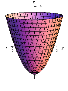
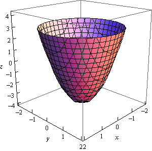
This is an elliptic paraboloid and is an example of a quadric surface. We saw several of these in the previous section. We will be seeing quadric surfaces fairly regularly later on in Calculus III.
Another common graph that we’ll be seeing quite a bit in this course is the graph of a plane. We have a convention for graphing planes that will make them a little easier to graph and hopefully visualize.
Recall that the equation of a plane is given by
\[ax + by + cz = d\]or if we solve this for \(z\) we can write it in terms of function notation. This gives,
\[f\left( {x,y} \right) = Ax + By + D\]To graph a plane we will generally find the intersection points with the three axes and then graph the triangle that connects those three points. This triangle will be a portion of the plane and it will give us a fairly decent idea on what the plane itself should look like. For example, let’s graph the plane given by,
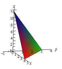
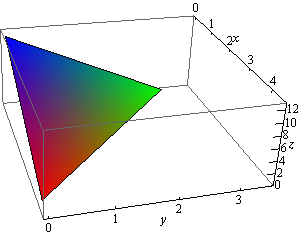
\[f\left( {x,y} \right) = 12 - 3x - 4y\]For purposes of graphing this it would probably be easier to write this as,
\[z = 12 - 3x - 4y\hspace{0.25in} \Rightarrow \hspace{0.25in}\,\,\,\,\,3x + 4y + z = 12\]Now, each of the intersection points with the three main coordinate axes is defined by the fact that two of the coordinates are zero. For instance, the intersection with the \(z\)-axis is defined by \(x = y = 0\). So, the three intersection points are,
\[\begin{align*}& x - {\mbox{axis : }}\left( {4,0,0} \right)\\ & y - {\mbox{axis : }}\left( {0,3,0} \right)\\ & z - {\mbox{axis : }}\left( {0,0,12} \right)\hspace{0.25in}\end{align*}\]Here is the graph of the plane.
Now, to extend this out, graphs of functions of the form \(w = f\left( {x,y,z} \right)\) would be four dimensional surfaces. Of course, we can’t graph them, but it doesn’t hurt to point this out.
We next want to talk about the domains of functions of more than one variable. Recall that domains of functions of a single variable, \(y = f\left( x \right)\), consisted of all the values of \(x\) that we could plug into the function and get back a real number. Now, if we think about it, this means that the domain of a function of a single variable is an interval (or intervals) of values from the number line, or one dimensional space.
The domain of functions of two variables, \(z = f\left( {x,y} \right)\), are regions from two dimensional space and consist of all the coordinate pairs, \(\left( {x,y} \right)\), that we could plug into the function and get back a real number.
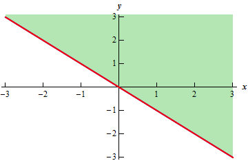
- \(f\left( {x,y} \right) = \sqrt {x + y} \)
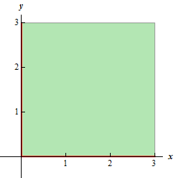
- \(f\left( {x,y} \right) = \sqrt x + \sqrt y \)
- \(f\left( {x,y} \right) = \ln \left( {9 - {x^2} - 9{y^2}} \right)\)
In this case we know that we can’t take the square root of a negative number so this means that we must require,
\[x + y \ge 0\]Here is a sketch of the graph of this region.
b \(f\left( {x,y} \right) = \sqrt x + \sqrt y \) Show Solution
This function is different from the function in the previous part. Here we must require that,
\[x \ge 0\hspace{0.25in}{\mbox{and}}\,\,\,\,\,y \ge 0\]and they really do need to be separate inequalities. There is one for each square root in the function. Here is the sketch of this region.
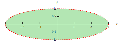
c \(f\left( {x,y} \right) = \ln \left( {9 - {x^2} - 9{y^2}} \right)\) Show Solution
In this final part we know that we can’t take the logarithm of a negative number or zero. Therefore, we need to require that,
\[9 - {x^2} - 9{y^2} > 0\hspace{0.25in} \Rightarrow \hspace{0.25in}\,\,\,\frac{{{x^2}}}{9} + {y^2} < 1\]and upon rearranging we see that we need to stay interior to an ellipse for this function. Here is a sketch of this region.
Note that domains of functions of three variables, \(w = f\left( {x,y,z} \right)\), will be regions in three dimensional space.
In this case we have to deal with the square root and division by zero issues. These will require,
\[{x^2} + {y^2} + {z^2} - 16 > 0\hspace{0.25in}\,\,\,\,\, \Rightarrow \hspace{0.25in}\,\,\,{x^2} + {y^2} + {z^2} > 16\]So, the domain for this function is the set of points that lies completely outside a sphere of radius 4 centered at the origin.
The next topic that we should look at is that of level curves or contour curves. The level curves of the function \(z = f\left( {x,y} \right)\) are two dimensional curves we get by setting \(z = k\), where \(k\) is any number. So the equations of the level curves are \(f\left( {x,y} \right) = k\). Note that sometimes the equation will be in the form \(f\left( {x,y,z} \right) = 0\) and in these cases the equations of the level curves are \(f\left( {x,y,k} \right) = 0\).
You’ve probably seen level curves (or contour curves, whatever you want to call them) before. If you’ve ever seen the elevation map for a piece of land, this is nothing more than the contour curves for the function that gives the elevation of the land in that area. Of course, we probably don’t have the function that gives the elevation, but we can at least graph the contour curves.
Let’s do a quick example of this.
First, for the sake of practice, let’s identify what this surface given by \(f\left( {x,y} \right)\) is. To do this let’s rewrite it as,
\[z = \sqrt {{x^2} + {y^2}} \]Recall from the Quadric Surfaces section that this the upper portion of the “cone” (or hour glass shaped surface).
Note that this was not required for this problem. It was done for the practice of identifying the surface and this may come in handy down the road.
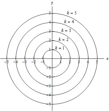
Now on to the real problem. The level curves (or contour curves) for this surface are given by the equation are found by substituting \(z = k\). In the case of our example this is,
\[k = \sqrt {{x^2} + {y^2}} \hspace{0.25in}\hspace{0.25in} \Rightarrow \hspace{0.25in}\hspace{0.25in}{x^2} + {y^2} = {k^2}\]where \(k\) is any number. So, in this case, the level curves are circles of radius \(k\) with center at the origin.
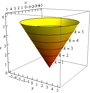
We can graph these in one of two ways. We can either graph them on the surface itself or we can graph them in a two dimensional axis system. Here is each graph for some values of \(k\).
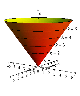
Note that we can think of contours in terms of the intersection of the surface that is given by \(z = f\left( {x,y} \right)\) and the plane \(z = k\). The contour will represent the intersection of the surface and the plane.
For functions of the form \(f\left( {x,y,z} \right)\) we will occasionally look at level surfaces. The equations of level surfaces are given by \(f\left( {x,y,z} \right) = k\) where \(k\) is any number.
The final topic in this section is that of traces. In some ways these are similar to contours. As noted above we can think of contours as the intersection of the surface given by \(z = f\left( {x,y} \right)\) and the plane \(z = k\). Traces of surfaces are curves that represent the intersection of the surface and the plane given by \(x = a\) or \(y = b\).
Let’s take a quick look at an example of traces.
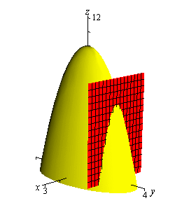
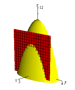
We’ll start with \(x = 1\). We can get an equation for the trace by plugging \(x = 1\) into the equation. Doing this gives,
\[z = f\left( {1,y} \right) = 10 - 4{\left( 1 \right)^2} - {y^2}\hspace{0.25in}\,\,\,\, \Rightarrow \hspace{0.25in}\,\,\,z = 6 - {y^2}\]and this will be graphed in the plane given by \(x = 1\).
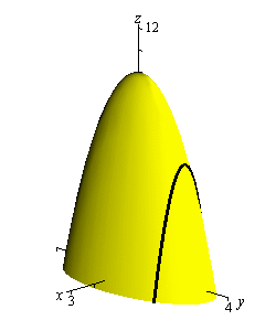
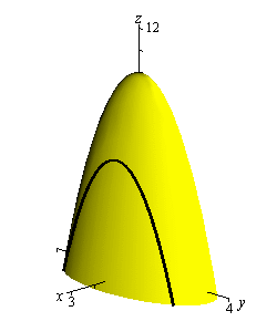
Below are two graphs. The graph on the left is a graph showing the intersection of the surface and the plane given by \(x = 1\). On the right is a graph of the surface and the trace that we are after in this part.
For \(y = 2\) we will do pretty much the same thing that we did with the first part. Here is the equation of the trace,
\[z = f\left( {x,2} \right) = 10 - 4{x^2} - {\left( 2 \right)^2}\hspace{0.25in}\,\,\,\, \Rightarrow \hspace{0.25in}\,\,\,z = 6 - 4{x^2}\]and here are the sketches for this case.