Section 9.1 : Parametric Equations and Curves
To this point (in both Calculus I and Calculus II) we’ve looked almost exclusively at functions in the form \(y = f\left( x \right)\) or \(x = h\left( y \right)\) and almost all of the formulas that we’ve developed require that functions be in one of these two forms. The problem is that not all curves or equations that we’d like to look at fall easily into this form.
Take, for example, a circle. It is easy enough to write down the equation of a circle centered at the origin with radius \(r\).
\[{x^2} + {y^2} = {r^2}\]However, we will never be able to write the equation of a circle down as a single equation in either of the forms above. Sure we can solve for \(x\) or \(y\) as the following two formulas show
\[y = \pm \sqrt {{r^2} - {x^2}} \hspace{0.5in}\hspace{0.25in}x = \pm \sqrt {{r^2} - {y^2}} \]but there are in fact two functions in each of these. Each formula gives a portion of the circle.
\[\begin{align*}y & = \sqrt {{r^2} - {x^2}} & \hspace{0.15in} & \left( {{\mbox{top}}} \right) \hspace{0.75in}\ & x & = \sqrt {{r^2} - {y^2}} & \hspace{0.15in} & \left( {{\mbox{right side}}} \right)\\ y & = - \sqrt {{r^2} - {x^2}} & \hspace{0.15in} & \left( {{\mbox{bottom}}} \right)\hspace{0.75in} & x & = - \sqrt {{r^2} - {y^2}} & \hspace{0.15in} & \left( {{\mbox{left side}}} \right)\end{align*}\]Unfortunately, we usually are working on the whole circle, or simply can’t say that we’re going to be working only on one portion of it. Even if we can narrow things down to only one of these portions the function is still often fairly unpleasant to work with.
There are also a great many curves out there that we can’t even write down as a single equation in terms of only \(x\) and \(y\). So, to deal with some of these problems we introduce parametric equations. Instead of defining \(y\) in terms of \(x\) (\(y = f\left( x \right)\)) or \(x\) in terms of \(y\) (\(x = h\left( y \right)\)) we define both \(x\) and \(y\) in terms of a third variable called a parameter as follows,
\[x = f\left( t \right)\hspace{0.5in}y = g\left( t \right)\]This third variable is usually denoted by \(t\) (as we did here) but doesn’t have to be of course. Sometimes we will restrict the values of \(t\) that we’ll use and at other times we won’t. This will often be dependent on the problem and just what we are attempting to do.
Each value of \(t\) defines a point \(\left( {x,y} \right) = \left( {f\left( t \right),g\left( t \right)} \right)\) that we can plot. The collection of points that we get by letting \(t\) be all possible values is the graph of the parametric equations and is called the parametric curve.
To help visualize just what a parametric curve is pretend that we have a big tank of water that is in constant motion and we drop a ping pong ball into the tank. The point \(\left( {x,y} \right) = \left( {f\left( t \right),g\left( t \right)} \right)\) will then represent the location of the ping pong ball in the tank at time \(t\) and the parametric curve will be a trace of all the locations of the ping pong ball. Note that this is not always a correct analogy but it is useful initially to help visualize just what a parametric curve is.
Sketching a parametric curve is not always an easy thing to do. Let’s take a look at an example to see one way of sketching a parametric curve. This example will also illustrate why this method is usually not the best.
At this point our only option for sketching a parametric curve is to pick values of \(t\), plug them into the parametric equations and then plot the points. So, let’s plug in some \(t\)’s.
| \(t\) | \(x\) | \(y\) |
|---|---|---|
| -2 | 2 | -5 |
| -1 | 0 | -3 |
| \( - \frac{1}{2}\) | \( - \frac{1}{4}\) | -2 |
| 0 | 0 | -1 |
| 1 | 2 | 1 |
The first question that should be asked at this point is, how did we know to use the values of \(t\) that we did, especially the third choice? Unfortunately, there is no real answer to this question at this point. We simply pick \(t\)’s until we are fairly confident that we’ve got a good idea of what the curve looks like. It is this problem with picking “good” values of \(t\) that make this method of sketching parametric curves one of the poorer choices. Sometimes we have no choice, but if we do have a choice we should avoid it.
We’ll discuss an alternate graphing method in later examples that will help to explain how these values of \(t\) were chosen.
We have one more idea to discuss before we actually sketch the curve. Parametric curves have a direction of motion. The direction of motion is given by increasing \(t\). So, when plotting parametric curves, we also include arrows that show the direction of motion. We will often give the value of \(t\) that gave specific points on the graph as well to make it clear the value of \(t\) that gave that particular point.
Here is the sketch of this parametric curve.
So, it looks like we have a parabola that opens to the right.
Before we end this example there is a somewhat important and subtle point that we need to discuss first. Notice that we made sure to include a portion of the sketch to the right of the points corresponding to \(t = - 2\) and \(t = 1\) to indicate that there are portions of the sketch there. Had we simply stopped the sketch at those points we are indicating that there was no portion of the curve to the right of those points and there clearly will be. We just didn’t compute any of those points.
This may seem like an unimportant point, but as we’ll see in the next example it’s more important than we might think.
Before addressing a much easier way to sketch this graph let’s first address the issue of limits on the parameter. In the previous example we didn’t have any limits on the parameter. Without limits on the parameter the graph will continue in both directions as shown in the sketch above.
We will often have limits on the parameter however and this will affect the sketch of the parametric equations. To see this effect let’s look a slight variation of the previous example.
Note that the only difference here is the presence of the limits on \(t\). All these limits do is tell us that we can’t take any value of \(t\) outside of this range. Therefore, the parametric curve will only be a portion of the curve above. Here is the parametric curve for this example.
Notice that with this sketch we started and stopped the sketch right on the points originating from the end points of the range of \(t\)’s. Contrast this with the sketch in the previous example where we had a portion of the sketch to the right of the “start” and “end” points that we computed.
In this case the curve starts at \(t = - 1\) and ends at \(t = 1\), whereas in the previous example the curve didn’t really start at the right most points that we computed. We need to be clear in our sketches if the curve starts/ends right at a point, or if that point was simply the first/last one that we computed.
It is now time to take a look at an easier method of sketching this parametric curve. This method uses the fact that in many, but not all, cases we can actually eliminate the parameter from the parametric equations and get a function involving only \(x\) and \(y\). We will sometimes call this the algebraic equation to differentiate it from the original parametric equations. There will be two small problems with this method, but it will be easy to address those problems. It is important to note however that we won’t always be able to do this.
Just how we eliminate the parameter will depend upon the parametric equations that we’ve got. Let’s see how to eliminate the parameter for the set of parametric equations that we’ve been working with to this point.
One of the easiest ways to eliminate the parameter is to simply solve one of the equations for the parameter (\(t\), in this case) and substitute that into the other equation. Note that while this may be the easiest to eliminate the parameter, it’s usually not the best way as we’ll see soon enough.
In this case we can easily solve \(y\) for \(t\).
\[t = \frac{1}{2}\left( {y + 1} \right)\]Plugging this into the equation for \(x\) gives the following algebraic equation,
\[x = {\left( {\frac{1}{2}\left( {y + 1} \right)} \right)^2} + \frac{1}{2}\left( {y + 1} \right) = \frac{1}{4}{y^2} + y + \frac{3}{4}\]Sure enough from our Algebra knowledge we can see that this is a parabola that opens to the right and will have a vertex at \(\left( { - \frac{1}{4}, - 2} \right)\).
We won’t bother with a sketch for this one as we’ve already sketched this once and the point here was more to eliminate the parameter anyway.
Before we leave this example let’s address one quick issue.
In the first example we just, seemingly randomly, picked values of \(t\) to use in our table, especially the third value. There really was no apparent reason for choosing \(t = - \frac{1}{2}\). It is however probably the most important choice of \(t\) as it is the one that gives the vertex.
The reality is that when writing this material up we actually did this problem first then went back and did the first problem. Plotting points is generally the way most people first learn how to construct graphs and it does illustrate some important concepts, such as direction, so it made sense to do that first in the notes. In practice however, this example is often done first.
So, how did we get those values of \(t\)? Well let’s start off with the vertex as that is probably the most important point on the graph. We have the \(x\) and \(y\) coordinates of the vertex and we also have \(x\) and \(y\) parametric equations for those coordinates. So, plug in the coordinates for the vertex into the parametric equations and solve for \(t\). Doing this gives,
\[\begin{array}{ll}{ - \frac{1}{4} = {t^2} + t}\\{ - 2 = 2t - 1}\end{array}\hspace{0.5in} \Rightarrow \hspace{0.5in}\begin{array}{ll}{t = - \frac{1}{2}\,\,\,\left( {{\mbox{double root}}} \right)}\\{t = - \frac{1}{2}}\end{array}\]So, as we can see, the value of \(t\) that will give both of these coordinates is \(t = - \frac{1}{2}\). Note that the \(x\) parametric equation gave a double root and this will often not happen. Often we would have gotten two distinct roots from that equation. In fact, it won’t be unusual to get multiple values of \(t\) from each of the equations.
However, what we can say is that there will be a value(s) of \(t\) that occurs in both sets of solutions and that is the \(t\) that we want for that point. We’ll eventually see an example where this happens in a later section.
Now, from this work we can see that if we use \(t = - \frac{1}{2}\) we will get the vertex and so we included that value of \(t\) in the table in Example 1. Once we had that value of \(t\) we chose two integer values of \(t\) on either side to finish out the table.
As we will see in later examples in this section determining values of \(t\) that will give specific points is something that we’ll need to do on a fairly regular basis. It is fairly simple however as this example has shown. All we need to be able to do is solve a (usually) fairly basic equation which by this point in time shouldn’t be too difficult.
Getting a sketch of the parametric curve once we’ve eliminated the parameter seems fairly simple. All we need to do is graph the equation that we found by eliminating the parameter. As noted already however, there are two small problems with this method. The first is direction of motion. The equation involving only \(x\) and \(y\) will NOT give the direction of motion of the parametric curve. This is generally an easy problem to fix however. Let’s take a quick look at the derivatives of the parametric equations from the last example. They are,
\[\begin{align*}\frac{{dx}}{{dt}} & = 2t + 1\\ \frac{{dy}}{{dt}} & = 2\end{align*}\]Now, all we need to do is recall our Calculus I knowledge. The derivative of \(y\) with respect to \(t\) is clearly always positive. Recalling that one of the interpretations of the first derivative is rate of change we now know that as \(t\) increases \(y\) must also increase. Therefore, we must be moving up the curve from bottom to top as \(t\) increases as that is the only direction that will always give an increasing \(y\) as \(t\) increases.
Note that the \(x\) derivative isn’t as useful for this analysis as it will be both positive and negative and hence \(x\) will be both increasing and decreasing depending on the value of \(t\). That doesn’t help with direction much as following the curve in either direction will exhibit both increasing and decreasing \(x\).
In some cases, only one of the equations, such as this example, will give the direction while in other cases either one could be used. It is also possible that, in some cases, both derivatives would be needed to determine direction. It will always be dependent on the individual set of parametric equations.
The second problem with eliminating the parameter is best illustrated in an example as we’ll be running into this problem in the remaining examples.
Before we proceed with eliminating the parameter for this problem let’s first address again why just picking \(t\)’s and plotting points is not really a good idea.
Given the range of \(t\)’s in the problem statement let’s use the following set of \(t\)’s.
| \(t\) | \(x\) | \(y\) |
|---|---|---|
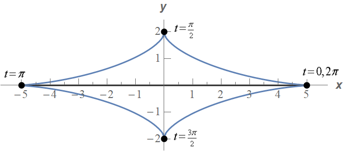
| 0 | 5 | 0 |
| \(\frac{\pi }{2}\) | 0 | 2 |
| \(\pi \) | -5 | 0 |
| \(\frac{{3\pi }}{2}\) | 0 | -2 |
| \(2\pi \) | 5 | 0 |
The question that we need to ask now is do we have enough points to accurately sketch the graph of this set of parametric equations? Below are some sketches of some possible graphs of the parametric equation based only on these five points.
Given the nature of sine/cosine you might be tempted to eliminate the diamond and the square but there is no denying that they are graphs that go through the given points. The first and fourth graphs both have some curvature to them and so you might be tempted to assume that one of those is the correct one given the sine/cosine in the equations. The last graph is also a little silly but it does show a graph going through the given points.
Again, given the nature of sine/cosine you are probably guessing that the correct graph is the the first or third graph. However, that is all that would be at this point. A guess. Nothing actually says unequivocally that the parametric curve is an will be one of those two just from those five points. That is the danger of sketching parametric curves based on a handful of points. Unless we know what the graph will be ahead of time we are really just making a guess.
It is important to note at this point that it is very easy to construct a set of parametric equations both containing sines and/or cosines and yet have the graph not have any curvature at all. You can often make some guesses as to the shape of the curve from the parametric equations but you won't always guess correctly unfortunately. Care must be taken when graphing parametric equations to not take the behavior of the individual parametric equations and just assume that behavior will translate to the curve of the set of parametric equations.
Also, in general, we should avoid plotting points to sketch parametric curves as that will, on occasion, lead to incorrect graphs. The best method, provided it can be done, is to eliminate the parameter. As noted just prior to starting this example there is still a potential problem with eliminating the parameter that we'll need to deal with. We will eventually discuss this issue. For now, let's just proceed with eliminating the parameter.
We’ll start by eliminating the parameter as we did in the previous section. We’ll solve one of the of the equations for \(t\) and plug this into the other equation. For example, we could do the following,
\[t = {\cos ^{ - 1}}\left( {\frac{x}{5}} \right)\hspace{0.5in} \Rightarrow \hspace{0.5in}y = 2\sin \left( {{{\cos }^{ - 1}}\left( {\frac{x}{5}} \right)} \right)\]Can you see the problem with doing this? This is definitely easy to do but we have a greater chance of correctly graphing the original parametric equations by plotting points than we do graphing this!
There are many ways to eliminate the parameter from the parametric equations and solving for \(t\) is usually not the best way to do it. While it is often easy to do we will, in most cases, end up with an equation that is almost impossible to deal with.
So, how can we eliminate the parameter here? In this case all we need to do is recall a very nice trig identity and the equation of an ellipse. Recall,
\[{\cos ^2}t + {\sin ^2}t = 1\]Then from the parametric equations we get,
\[\cos t = \frac{x}{5}\hspace{0.5in}\sin t = \frac{y}{2}\]Then, using the trig identity from above and these equations we get,
\[1 = {\cos ^2}t + {\sin ^2}t = {\left( {\frac{x}{5}} \right)^2} + {\left( {\frac{y}{2}} \right)^2} = \frac{{{x^2}}}{{25}} + \frac{{{y^2}}}{4}\]So we now know that we will have an ellipse.
Now, let’s continue on with the example. We’ve identified that the parametric equations describe an ellipse, but we can’t just sketch an ellipse and be done with it.
First, just because the algebraic equation was an ellipse doesn’t actually mean that the parametric curve is the full ellipse. It is always possible that the parametric curve is only a portion of the ellipse. In order to identify just how much of the ellipse the parametric curve will cover let’s go back to the parametric equations and see what they tell us about any limits on \(x\) and \(y\). Based on our knowledge of sine and cosine we have the following,
\[\begin{align*} & - 1 \le \cos t \le 1\hspace{0.25in} \Rightarrow \hspace{0.25in} - 5 \le 5\cos t \le 5\hspace{0.25in} \Rightarrow \hspace{0.25in}\,\, - 5 \le x \le 5\\ & - 1 \le \sin t \le 1\hspace{0.25in} \Rightarrow \hspace{0.25in} - 2 \le 2\sin t \le 2 \,\hspace{0.25in} \Rightarrow \hspace{0.25in}\,\, - 2 \le y \le 2\end{align*}\]So, by starting with sine/cosine and “building up” the equation for \(x\) and \(y\) using basic algebraic manipulations we get that the parametric equations enforce the above limits on \(x\) and \(y\). In this case, these also happen to be the full limits on \(x\) and \(y\) we get by graphing the full ellipse.
This is the second potential issue alluded to above. The parametric curve may not always trace out the full graph of the algebraic curve. We should always find limits on \(x\) and \(y\) enforced upon us by the parametric curve to determine just how much of the algebraic curve is actually sketched out by the parametric equations.
Therefore, in this case, we now know that we get a full ellipse from the parametric equations. Before we proceed with the rest of the example be careful to not always just assume we will get the full graph of the algebraic equation. There are definitely times when we will not get the full graph and we’ll need to do a similar analysis to determine just how much of the graph we actually get. We’ll see an example of this later.
Note as well that any limits on \(t\) given in the problem statement can also affect how much of the graph of the algebraic equation we get. In this case however, based on the table of values we computed at the start of the problem we can see that we do indeed get the full ellipse in the range \(0 \le t \le 2\pi \). That won’t always be the case however, so pay attention to any restrictions on \(t\) that might exist!
Next, we need to determine a direction of motion for the parametric curve. Recall that all parametric curves have a direction of motion and the equation of the ellipse simply tells us nothing about the direction of motion.
To get the direction of motion it is tempting to just use the table of values we computed above to get the direction of motion. In this case, we would guess (and yes that is all it is – a guess) that the curve traces out in a counter-clockwise direction. We’d be correct. In this case, we’d be correct! The problem is that tables of values can be misleading when determining a direction of motion as we’ll see in the next example.
Therefore, it is best to not use a table of values to determine the direction of motion. To correctly determine the direction of motion we’ll use the same method of determining the direction that we discussed after Example 3. In other words, we’ll take the derivative of the parametric equations and use our knowledge of Calculus I and trig to determine the direction of motion.
The derivatives of the parametric equations are,
\[\frac{{dx}}{{dt}} = - 5\sin t\hspace{0.5in}\frac{{dy}}{{dt}} = 2\cos t\]Now, at \(t = 0\) we are at the point \(\left( {5,0} \right)\) and let’s see what happens if we start increasing \(t\). Let’s increase \(t\) from \(t = 0\) to \(t = \frac{\pi }{2}\). In this range of \(t\)’s we know that sine is always positive and so from the derivative of the \(x\) equation we can see that \(x\) must be decreasing in this range of \(t\)’s.
This, however, doesn’t really help us determine a direction for the parametric curve. Starting at \(\left( {5,0} \right)\) no matter if we move in a clockwise or counter-clockwise direction \(x\) will have to decrease so we haven’t really learned anything from the \(x\) derivative.
The derivative from the \(y\) parametric equation on the other hand will help us. Again, as we increase \(t\) from \(t = 0\) to \(t = \frac{\pi }{2}\) we know that cosine will be positive and so \(y\) must be increasing in this range. That however, can only happen if we are moving in a counter‑clockwise direction. If we were moving in a clockwise direction from the point \(\left( {5,0} \right)\) we can see that \(y\) would have to decrease!
Therefore, in the first quadrant we must be moving in a counter-clockwise direction. Let’s move on to the second quadrant.
So, we are now at the point \(\left( {0,2} \right)\) and we will increase \(t\) from \(t = \frac{\pi }{2}\) to \(t = \pi \). In this range of \(t\) we know that cosine will be negative and sine will be positive. Therefore, from the derivatives of the parametric equations we can see that \(x\) is still decreasing and \(y\) will now be decreasing as well.
In this quadrant the \(y\) derivative tells us nothing as \(y\) simply must decrease to move from \(\left( {0,2} \right)\). However, in order for \(x\) to decrease, as we know it does in this quadrant, the direction must still be moving a counter-clockwise rotation.
We are now at \(\left( { - 5,0} \right)\) and we will increase \(t\) from \(t = \pi \) to \(t = \frac{{3\pi }}{2}\). In this range of \(t\) we know that cosine is negative (and hence \(y\) will be decreasing) and sine is also negative (and hence \(x\) will be increasing). Therefore, we will continue to move in a counter‑clockwise motion.
For the 4th quadrant we will start at \(\left( {0, - 2} \right)\) and increase \(t\) from \(t = \frac{{3\pi }}{2}\) to \(t = 2\pi \). In this range of \(t\) we know that cosine is positive (and hence \(y\) will be increasing) and sine is negative (and hence \(x\) will be increasing). So, as in the previous three quadrants, we continue to move in a counter‑clockwise motion.
At this point we covered the range of \(t\)’s we were given in the problem statement and during the full range the motion was in a counter-clockwise direction.
We can now fully sketch the parametric curve so, here is the sketch.
Okay, that was a really long example. Most of these types of problems aren’t as long. We just had a lot to discuss in this one so we could get a couple of important ideas out of the way. The rest of the examples in this section shouldn’t take as long to go through.
Now, let’s take a look at another example that will illustrate an important idea about parametric equations.
Note that the only difference in between these parametric equations and those in Example 4 is that we replaced the \(t\) with 3\(t\). We can eliminate the parameter here in the same manner as we did in the previous example.
\[\cos \left( {3t} \right) = \frac{x}{5}\hspace{0.5in}\sin \left( {3t} \right) = \frac{y}{2}\]We then get,
\[1 = {\cos ^2}\left( {3t} \right) + {\sin ^2}\left( {3t} \right) = {\left( {\frac{x}{5}} \right)^2} + {\left( {\frac{y}{2}} \right)^2} = \frac{{{x^2}}}{{25}} + \frac{{{y^2}}}{4}\]So, we get the same ellipse that we did in the previous example. Also note that we can do the same analysis on the parametric equations to determine that we have exactly the same limits on \(x\) and \(y\). Namely,
\[ - 5 \le x \le 5\hspace{0.5in}\hspace{0.25in} - 2 \le y \le 2\]It’s starting to look like changing the \(t\) into a 3\(t\) in the trig equations will not change the parametric curve in any way. That is not correct however. The curve does change in a small but important way which we will be discussing shortly.
Before discussing that small change the 3\(t\) brings to the curve let’s discuss the direction of motion for this curve. Despite the fact that we said in the last example that picking values of \(t\) and plugging in to the equations to find points to plot is a bad idea let’s do it any way.
Given the range of \(t\)’s from the problem statement the following set looks like a good choice of \(t\)’s to use.
| \(t\) | \(x\) | \(y\) |
|---|---|---|
| 0 | 5 | 0 |
| \(\frac{\pi }{2}\) | 0 | -2 |
| \(\pi \) | -5 | 0 |
| \(\frac{{3\pi }}{2}\) | 0 | 2 |
| \(2\pi \) | 5 | 0 |
So, the only change to this table of values/points from the last example is all the nonzero \(y\) values changed sign. From a quick glance at the values in this table it would look like the curve, in this case, is moving in a clockwise direction. But is that correct? Recall we said that these tables of values can be misleading when used to determine direction and that’s why we don’t use them.
Let’s see if our first impression is correct. We can check our first impression by doing the derivative work to get the correct direction. Let’s work with just the \(y\) parametric equation as the \(x\) will have the same issue that it had in the previous example. The derivative of the \(y\) parametric equation is,
\[\frac{{dy}}{{dt}} = 6\cos \left( {3t} \right)\]Now, if we start at \(t = 0\) as we did in the previous example and start increasing \(t\). At \(t = 0\) the derivative is clearly positive and so increasing \(t\) (at least initially) will force \(y\) to also be increasing. The only way for this to happen is if the curve is in fact tracing out in a counter-clockwise direction initially.
Now, we could continue to look at what happens as we further increase \(t\), but when dealing with a parametric curve that is a full ellipse (as this one is) and the argument of the trig functions is of the form nt for any constant \(n\) the direction will not change so once we know the initial direction we know that it will always move in that direction. Note that this is only true for parametric equations in the form that we have here. We’ll see in later examples that for different kinds of parametric equations this may no longer be true.
Okay, from this analysis we can see that the curve must be traced out in a counter‑clockwise direction. This is directly counter to our guess from the tables of values above and so we can see that, in this case, the table would probably have led us to the wrong direction. So, once again, tables are generally not very reliable for getting pretty much any real information about a parametric curve other than a few points that must be on the curve. Outside of that the tables are rarely useful and will generally not be dealt with in further examples.
So, why did our table give an incorrect impression about the direction? Well recall that we mentioned earlier that the 3\(t\) will lead to a small but important change to the curve versus just a \(t\)? Let’s take a look at just what that change is as it will also answer what “went wrong” with our table of values.
Let’s start by looking at \(t = 0\). At \(t = 0\) we are at the point \(\left( {5,0} \right)\) and let’s ask ourselves what values of \(t\) put us back at this point. We saw in Example 3 how to determine value(s) of \(t\) that put us at certain points and the same process will work here with a minor modification.
Instead of looking at both the \(x\) and \(y\) equations as we did in that example let’s just look at the \(x\) equation. The reason for this is that we’ll note that there are two points on the ellipse that will have a \(y\) coordinate of zero, \(\left( {5,0} \right)\) and \(\left( { - 5,0} \right)\). If we set the \(y\) coordinate equal to zero we’ll find all the \(t\)’s that are at both of these points when we only want the values of \(t\) that are at \(\left( {5,0} \right)\).
So, because the \(x\) coordinate of five will only occur at this point we can simply use the \(x\) parametric equation to determine the values of \(t\) that will put us at this point. Doing this gives the following equation and solution,
\[\begin{align*}5 & = 5\cos \left( {3t} \right)\,\\ 3t & = {\cos ^{ - 1}}\left( 1 \right) = 0 + 2\pi n\hspace{0.25in}\,\,\, \to \hspace{0.25in}\,\,\,\,\,\,t = \frac{2}{3}\pi n\,\,\,\,\,\,n = 0, \pm 1, \pm 2, \pm 3, \ldots \end{align*}\]Don’t forget that when solving a trig equation we need to add on the “\( + 2\pi n\)” where \(n\) represents the number of full revolutions in the counter-clockwise direction (positive \(n\)) and clockwise direction (negative \(n\)) that we rotate from the first solution to get all possible solutions to the equation.
Now, let’s plug in a few values of \(n\) starting at \(n = 0\). We don’t need negative \(n\) in this case since all of those would result in negative \(t\) and those fall outside of the range of \(t\)’s we were given in the problem statement. The first few values of \(t\) are then,
\[\begin{align*}n & = 0\hspace{0.25in} : \hspace{0.25in} t = 0\\ n & = 1\hspace{0.25in}:\hspace{0.25in}t = \frac{{2\pi }}{3}\\ n & = 2\hspace{0.25in}:\hspace{0.25in}t = \frac{{4\pi }}{3}\\ n & = 3\hspace{0.25in}:\hspace{0.25in}t = \frac{{6\pi }}{3} = 2\pi \end{align*}\]We can stop here as all further values of \(t\) will be outside the range of \(t\)’s given in this problem.
So, what is this telling us? Well back in Example 4 when the argument was just \(t\) the ellipse was traced out exactly once in the range \(0 \le t \le 2\pi \). However, when we change the argument to 3\(t\) (and recalling that the curve will always be traced out in a counter‑clockwise direction for this problem) we are going through the “starting” point of \(\left( {5,0} \right)\) two more times than we did in the previous example.
In fact, this curve is tracing out three separate times. The first trace is completed in the range \(0 \le t \le \frac{{2\pi }}{3}\). The second trace is completed in the range \(\frac{{2\pi }}{3} \le t \le \frac{{4\pi }}{3}\) and the third and final trace is completed in the range \(\frac{{4\pi }}{3} \le t \le 2\pi \). In other words, changing the argument from \(t\) to 3\(t\) increase the speed of the trace and the curve will now trace out three times in the range \(0 \le t \le 2\pi \)!
This is why the table gives the wrong impression. The speed of the tracing has increased leading to an incorrect impression from the points in the table. The table seems to suggest that between each pair of values of \(t\) a quarter of the ellipse is traced out in the clockwise direction when in reality it is tracing out three quarters of the ellipse in the counter-clockwise direction.
Here’s a final sketch of the curve and note that it really isn’t all that different from the previous sketch. The only differences are the values of \(t\) and the various points we included. We did include a few more values of \(t\) at various points just to illustrate where the curve is at for various values of \(t\) but in general these really aren’t needed.
So, we saw in the last two examples two sets of parametric equations that in some way gave the same graph. Yet, because they traced out the graph a different number of times we really do need to think of them as different parametric curves at least in some manner. This may seem like a difference that we don’t need to worry about, but as we will see in later sections this can be a very important difference. In some of the later sections we are going to need a curve that is traced out exactly once.
Before we move on to other problems let’s briefly acknowledge what happens by changing the \(t\) to an nt in these kinds of parametric equations. When we are dealing with parametric equations involving only sines and cosines and they both have the same argument if we change the argument from \(t\) to nt we simply change the speed with which the curve is traced out. If \(n > 1\) we will increase the speed and if \(n < 1\) we will decrease the speed.
Let’s take a look at a couple more examples.
We can eliminate the parameter much as we did in the previous two examples. However, we’ll need to note that the \(x\) already contains a \({\sin ^2}t\) and so we won’t need to square the \(x\). We will however, need to square the \(y\) as we need in the previous two examples.
\[x + \frac{{{y^2}}}{4} = {\sin ^2}t + {\cos ^2}t = 1\hspace{0.5in} \Rightarrow \hspace{0.5in}x = 1 - \frac{{{y^2}}}{4}\]In this case the algebraic equation is a parabola that opens to the left.
We will need to be very, very careful however in sketching this parametric curve. We will NOT get the whole parabola. A sketch of the algebraic form parabola will exist for all possible values of \(y\). However, the parametric equations have defined both \(x\) and \(y\) in terms of sine and cosine and we know that the ranges of these are limited and so we won’t get all possible values of \(x\) and \(y\) here. So, first let’s get limits on \(x\) and \(y\) as we did in previous examples. Doing this gives,
\[\begin{array}{ccccc} - 1 \le \sin t \le 1 & \hspace{0.25in}\Rightarrow \hspace{0.25in} & 0 \le {\sin ^2}t \le 1 & \hspace{0.25in} \Rightarrow \hspace{0.25in} & 0 \le x \le 1\\ - 1 \le \cos t \le 1 & \hspace{0.25in} \Rightarrow \hspace{0.25in} & - 2 \le 2\cos t \le 2 & \hspace{0.25in} \Rightarrow \hspace{0.25in} & - 2 \le y \le 2\end{array}\]So, it is clear from this that we will only get a portion of the parabola that is defined by the algebraic equation. Below is a quick sketch of the portion of the parabola that the parametric curve will cover.
To finish the sketch of the parametric curve we also need the direction of motion for the curve. Before we get to that however, let’s jump forward and determine the range of \(t\)’s for one trace. To do this we’ll need to know the \(t\)’s that put us at each end point and we can follow the same procedure we used in the previous example. The only difference is this time let’s use the \(y\) parametric equation instead of the \(x\) because the \(y\) coordinates of the two end points of the curve are different whereas the \(x\) coordinates are the same.
So, for the top point we have,
\[\begin{align*}2 & = 2\cos t\\ t & = {\cos ^{ - 1}}\left( 1 \right) = 0 + 2\pi n = 2\pi n,\hspace{0.25in}n = 0, \pm 1, \pm 2, \pm 3, \ldots \end{align*}\]For, plugging in some values of \(n\) we get that the curve will be at the top point at,
\[t = \ldots , - 4\pi , - 2\pi ,0,2\pi ,4\pi , \ldots \]Similarly, for the bottom point we have,
\[\begin{align*} - 2 & = 2\cos t\\ t & = {\cos ^{ - 1}}\left( { - 1} \right) = \pi + 2\pi n,\hspace{0.25in}n = 0, \pm 1, \pm 2, \pm 3, \ldots \end{align*}\]So, we see that we will be at the bottom point at,
\[t = \ldots , - 3\pi , - \pi ,\pi ,3\pi , \ldots \]So, if we start at say, \(t = 0\), we are at the top point and we increase \(t\) we have to move along the curve downwards until we reach \(t = \pi \) at which point we are now at the bottom point. This means that we will trace out the curve exactly once in the range \(0 \le t \le \pi \).
This is not the only range that will trace out the curve however. Note that if we further increase \(t\) from \(t = \pi \) we will now have to travel back up the curve until we reach \(t = 2\pi \) and we are now back at the top point. Increasing \(t\) again until we reach \(t = 3\pi \) will take us back down the curve until we reach the bottom point again, etc. From this analysis we can get two more ranges of \(t\) for one trace,
\[\pi \le t \le 2\pi \hspace{0.5in}2\pi \le t \le 3\pi \]As you can probably see there are an infinite number of ranges of \(t\) we could use for one trace of the curve. Any of them would be acceptable answers for this problem.
Note that in the process of determining a range of \(t\)’s for one trace we also managed to determine the direction of motion for this curve. In the range \(0 \le t \le \pi \) we had to travel downwards along the curve to get from the top point at \(t = 0\) to the bottom point at \(t = \pi \). However, at \(t = 2\pi \) we are back at the top point on the curve and to get there we must travel along the path. We can’t just jump back up to the top point or take a different path to get there. All travel must be done on the path sketched out. This means that we had to go back up the path. Further increasing \(t\) takes us back down the path, then up the path again etc.
In other words, this path is sketched out in both directions because we are not putting any restrictions on the \(t\)’s and so we have to assume we are using all possible values of \(t\). If we had put restrictions on which \(t\)’s to use we might really have ended up only moving in one direction. That however would be a result only of the range of \(t\)’s we are using and not the parametric equations themselves.
Note that we didn’t really need to do the above work to determine that the curve traces out in both directions.in this case. Both the \(x\) and \(y\) parametric equations involve sine or cosine and we know both of those functions oscillate. This, in turn means that both \(x\) and \(y\) will oscillate as well. The only way for that to happen on this particular this curve will be for the curve to be traced out in both directions.
Be careful with the above reasoning that the oscillatory nature of sine/cosine forces the curve to be traced out in both directions. It can only be used in this example because the “starting” point and “ending” point of the curves are in different places. The only way to get from one of the “end” points on the curve to the other is to travel back along the curve in the opposite direction.
Contrast this with the ellipse in Example 4. In that case we had sine/cosine in the parametric equations as well. However, the curve only traced out in one direction, not in both directions. In Example 4 we were graphing the full ellipse and so no matter where we start sketching the graph we will eventually get back to the “starting” point without ever retracing any portion of the graph. In Example 4 as we trace out the full ellipse both \(x\) and \(y\) do in fact oscillate between their two “endpoints” but the curve itself does not trace out in both directions for this to happen.
Basically, we can only use the oscillatory nature of sine/cosine to determine that the curve traces out in both directions if the curve starts and ends at different points. If the starting/ending point is the same then we generally need to go through the full derivative argument to determine the actual direction of motion.
So, to finish this problem out, below is a sketch of the parametric curve. Note that we put direction arrows in both directions to clearly indicate that it would be traced out in both directions. We also put in a few values of \(t\) just to help illustrate the direction of motion.
To this point we’ve seen examples that would trace out the complete graph that we got by eliminating the parameter if we took a large enough range of \(t\)’s. However, in the previous example we’ve now seen that this will not always be the case. It is more than possible to have a set of parametric equations which will continuously trace out just a portion of the curve. We can usually determine if this will happen by looking for limits on \(x\) and \(y\) that are imposed up us by the parametric equation.
We will often use parametric equations to describe the path of an object or particle. Let’s take a look at an example of that.
Completely describe the path of this particle. Do this by sketching the path, determining limits on \(x\) and \(y\) and giving a range of \(t\)’s for which the path will be traced out exactly once (provided it traces out more than once of course).
Eliminating the parameter this time will be a little different. We only have cosines this time and we’ll use that to our advantage. We can solve the \(x\) equation for cosine and plug that into the equation for \(y\). This gives,
\[\cos \left( {2t} \right) = \frac{x}{3}\hspace{0.5in}y = 1 + {\left( {\frac{x}{3}} \right)^2} = 1 + \frac{{{x^2}}}{9}\]This time the algebraic equation is a parabola that opens upward. We also have the following limits on \(x\) and \(y\).
\[\begin{array}{ccccc} - 1 \le \cos \left( {2t} \right) \le 1 & \hspace{0.25in} & - 3 \le 3\cos \left( {2t} \right) \le 3 & \hspace{0.5in} & - 3 \le x \le 3\\ 0 \le {\cos ^2}\left( {2t} \right) \le 1 & \hspace{0.25in} & 1 \le 1 + {\cos ^2}\left( {2t} \right) \le 2 & \hspace{0.25in} & 1 \le y \le 2\end{array}\]So, again we only trace out a portion of the curve. Here is a quick sketch of the portion of the parabola that the parametric curve will cover.
Now, as we discussed in the previous example because both the \(x\) and \(y\) parametric equations involve cosine we know that both \(x\) and \(y\) must oscillate and because the “start” and “end” points of the curve are not the same the only way \(x\) and \(y\) can oscillate is for the curve to trace out in both directions.
To finish the problem then all we need to do is determine a range of \(t\)’s for one trace. Because the “end” points on the curve have the same \(y\) value and different \(x\) values we can use the \(x\) parametric equation to determine these values. Here is that work.
\[\begin{array}{ll} \begin{aligned}x = 3: \\ \\ \\ \end{aligned} &\begin{aligned}3 & = 3\cos \left( {2t} \right)\\ 1 & = \cos \left( {2t} \right)\\ 2t & = 0 + 2\pi n\hspace{0.25in}\, \to \hspace{0.25in}t = \pi n\hspace{0.25in}\,\,\,n = 0, \pm 1, \pm 2, \pm 3, \ldots \end{aligned}\end{array}\] \[\begin{array}{ll}\begin{aligned}x = -3: \\ \\ \\ \\ \end{aligned} &\begin{aligned} - 3 & = 3\cos \left( {2t} \right)\\ - 1 & = \cos \left( {2t} \right)\\ 2t & = \pi + 2\pi n\hspace{0.25in}\, \to \hspace{0.25in}t = \frac{1}{2}\pi + \pi n\hspace{0.25in}\,\,\,n = 0, \pm 1, \pm 2, \pm 3, \ldots \end{aligned}\end{array}\]So, we will be at the right end point at \(t = \ldots , - 2\pi , - \pi ,0,\pi ,2\pi , \ldots \) and we’ll be at the left end point at \(t = \ldots , - \frac{3}{2}\pi , - \frac{1}{2}\pi ,\frac{1}{2}\pi ,\frac{3}{2}\pi , \ldots \) . So, in this case there are an infinite number of ranges of \(t\)’s for one trace. Here are a few of them.
\[ - \frac{1}{2}\pi \le t \le 0\hspace{0.25in}\hspace{0.25in}0 \le t \le \frac{1}{2}\pi \hspace{0.25in}\hspace{0.25in}\frac{1}{2}\pi \le t \le \pi \]Here is a final sketch of the particle’s path with a few values of \(t\) on it.
We should give a small warning at this point. Because of the ideas involved in them we concentrated on parametric curves that retraced portions of the curve more than once. Do not, however, get too locked into the idea that this will always happen. Many, if not most parametric curves will only trace out once. The first one we looked at is a good example of this. That parametric curve will never repeat any portion of itself.
There is one final topic to be discussed in this section before moving on. So far we’ve started with parametric equations and eliminated the parameter to determine the parametric curve.
However, there are times in which we want to go the other way. Given a function or equation we might want to write down a set of parametric equations for it. In these cases we say that we parameterize the function.
If we take Examples 4 and 5 as examples we can do this for ellipses (and hence circles). Given the ellipse
\[\frac{{{x^2}}}{{{a^2}}} + \frac{{{y^2}}}{{{b^2}}} = 1\]a set of parametric equations for it would be,
\[x = a\cos t\hspace{1.0in}y = b\sin t\]This set of parametric equations will trace out the ellipse starting at the point \(\left( {a,0} \right)\) and will trace in a counter-clockwise direction and will trace out exactly once in the range \(0 \le t \le 2\pi \). This is a fairly important set of parametric equations as it is used continually in some subjects with dealing with ellipses and/or circles.
Every curve can be parameterized in more than one way. Any of the following will also parameterize the same ellipse.
\[\begin{align*}x & = a\cos \left( {\omega \,t} \right)\hspace{0.5in} & y & = b\sin \left( {\omega \,t} \right)\\ x & = a\sin \left( {\omega \,t} \right)\hspace{0.5in} & y & = b\cos \left( {\omega \,t} \right)\\ x & = a\cos \left( {\omega \,t} \right)\hspace{0.5in} & y & = - b\sin \left( {\omega \,t} \right)\end{align*}\]The presence of the \(\omega \) will change the speed that the ellipse rotates as we saw in Example 5. Note as well that the last two will trace out ellipses with a clockwise direction of motion (you might want to verify this). Also note that they won’t all start at the same place (if we think of \(t = 0\) as the starting point that is).
There are many more parameterizations of an ellipse of course, but you get the idea. It is important to remember that each parameterization will trace out the curve once with a potentially different range of \(t\)’s. Each parameterization may rotate with different directions of motion and may start at different points.
You may find that you need a parameterization of an ellipse that starts at a particular place and has a particular direction of motion and so you now know that with some work you can write down a set of parametric equations that will give you the behavior that you’re after.
Now, let’s write down a couple of other important parameterizations and all the comments about direction of motion, starting point, and range of \(t\)’s for one trace (if applicable) are still true.
First, because a circle is nothing more than a special case of an ellipse we can use the parameterization of an ellipse to get the parametric equations for a circle centered at the origin of radius \(r\) as well. One possible way to parameterize a circle is,
\[x = r\cos t\hspace{1.0in}y = r\sin t\]Finally, even though there may not seem to be any reason to, we can also parameterize functions in the form \(y = f\left( x \right)\) or \(x = h\left( y \right)\). In these cases we parameterize them in the following way,
\[\begin{align*}x & = t\hspace{1.0in} & x & = h\left( t \right)\\ y & = f\left( t \right)\hspace{1.0in} & y & = t\end{align*}\]At this point it may not seem all that useful to do a parameterization of a function like this, but there are many instances where it will actually be easier, or it may even be required, to work with the parameterization instead of the function itself. Unfortunately, almost all of these instances occur in a Calculus III course.