Calculus III - Line Integrals

Show Mobile Notice Show All Notes Hide All Notes

Mobile Notice

You appear to be on a device with a "narrow" screen width (i.e. you are probably on a mobile phone). Due to the nature of the mathematics on this site it is best views in landscape mode. If your device is not in landscape mode many of the equations will run off the side of your device (should be able to scroll to see them) and some of the menu items will be cut off due to the narrow screen width.

Section 16.2 : Line Integrals - Part I

In this section we are now going to introduce a new kind of integral. However, before we do that it is important to note that you will need to remember how to parameterize equations, or put another way, you will need to be able to write down a set of parametric equations for a given curve. You should have seen some of this in your Calculus II course. If you need some review you should go back and review some of the basics of parametric equations and curves.

Here are some of the more basic curves that we’ll need to know how to do as well as limits on the parameter if they are required.

Curve	Parametric Equations
$\begin{array}{c} \displaystyle \frac{{{x^2}}}{{{a^2}}} + \frac{{{y^2}}}{{{b^2}}} = 1 \\ \mbox{(Ellipse)}\end{array}$	$\begin{array}{c} \begin{array}{c}\mbox{Counter-Clockwise} \\x = a\cos \left( t \right)\\ y = b\sin \left( t \right)\\ 0 \le t \le 2\pi \end{array}& \begin{array}{c} \mbox{Clockwise} \\x = a\cos \left( t \right)\\ y = - b\sin \left( t \right)\\ 0 \le t \le 2\pi \end{array} \end{array}$

$\begin{array}{c}{x^2} + {y^2} = {r^2} \\ \mbox{(Circle)}\end{array}$	$\begin{array}{c} \begin{array}{c}\mbox{Counter-Clockwise} \\ x = r\cos \left( t \right)\\ y = r\sin \left( t \right)\\ 0 \le t \le 2\pi \end{array} & \begin{array}{c} \mbox{Clockwise} \\ x = r\cos \left( t \right)\\ y = - r\sin \left( t \right)\\ 0 \le t \le 2\pi \end{array} \end{array}$

$y = f\left( x \right)$	$\begin{align}x & = t\\ y & = f\left( t \right)\end{align}$
$x = g\left( y \right)$	$\begin{align}x & = g\left( t \right)\\ y & = t\end{align}$

$\begin{array}{l}\mbox{Line Segment From} \\ \left( {{x_0},{y_0},{z_0}} \right) \mbox{ to} \\ \left( {{x_1},{y_1},{z_1}} \right) \end{array}$	$\begin{array}{c} \vec r\left( t \right) = \left( {1 - t} \right)\left\langle {{x_0},{y_0},{z_0}} \right\rangle + t\left\langle {{x_1},{y_1},{z_1}} \right\rangle \,\,\,,\,\,0 \le t \le 1 \\ \mbox{or} \\ \begin{array}{l} \begin{aligned} x & = \left( {1 - t} \right){x_0} + t\,{x_1}\\ y & = \left( {1 - t} \right){y_0} + t\,{y_1}\\ z & = \left( {1 - t} \right){z_0} + t\,{z_1} \end{aligned} & , \,\,\,\,\,\, 0 \le t \le 1 \end{array} \end{array}$

With the final one we gave both the vector form of the equation as well as the parametric form and if we need the two-dimensional version then we just drop the $z$ components. In fact, we will be using the two-dimensional version of this in this section.

For the ellipse and the circle we’ve given two parameterizations, one tracing out the curve clockwise and the other counter-clockwise. As we’ll eventually see the direction that the curve is traced out can, on occasion, change the answer. Also, both of these “start” on the positive $x$-axis at $t = 0$.

Now let’s move on to line integrals. In Calculus I we integrated $f\left( x \right)$, a function of a single variable, over an interval $\left[ {a,b} \right]$. In this case we were thinking of $x$ as taking all the values in this interval starting at $a$ and ending at $b$. With line integrals we will start with integrating the function $f\left( {x,y} \right)$, a function of two variables, and the values of $x$ and $y$ that we’re going to use will be the points, $\left( {x,y} \right)$, that lie on a curve $C$. Note that this is different from the double integrals that we were working with in the previous chapter where the points came out of some two-dimensional region.

Let’s start with the curve $C$ that the points come from. We will assume that the curve is smooth (defined shortly) and is given by the parametric equations,

\[x = h\left( t \right)\hspace{0.25in}y = g\left( t \right)\hspace{0.25in}\,\,\,\,a \le t \le b\]

We will often want to write the parameterization of the curve as a vector function. In this case the curve is given by,

\[\vec r\left( t \right) = h\left( t \right)\,\vec i + g\left( t \right)\vec j\hspace{0.25in}\hspace{0.25in}a \le t \le b\]

The curve is called smooth if $\vec r'\left( t \right)$ is continuous and $\vec r'\left( t \right) \ne 0$ for all $t$.

The line integral of $f\left( {x,y} \right)$ along $C$ is denoted by,

\[\int\limits_{C}{{f\left( {x,y} \right)\,ds}}\]

We use a $ds$ here to acknowledge the fact that we are moving along the curve, $C$, instead of the $x$-axis (denoted by $dx$) or the $y$-axis (denoted by $dy$). Because of the $ds$ this is sometimes called the line integral of $f$ with respect to arc length.

We’ve seen the notation $ds$ before. If you recall from Calculus II when we looked at the arc length of a curve given by parametric equations we found it to be,

\[L = \int_{{\,a}}^{{\,b}}{{ds}}\,\,,\hspace{0.25in}{\mbox{where }}ds = \sqrt {{{\left( {\frac{{dx}}{{dt}}} \right)}^2} + {{\left( {\frac{{dy}}{{dt}}} \right)}^2}} \,dt\]

It is no coincidence that we use $ds$ for both of these problems. The $ds$ is the same for both the arc length integral and the notation for the line integral.

So, to compute a line integral we will convert everything over to the parametric equations. The line integral is then,

\[\int\limits_{C}{{f\left( {x,y} \right)\,ds}} = \int_{{\,a}}^{{\,b}}{{f\left( {h\left( t \right),g\left( t \right)} \right)\sqrt {{{\left( {\frac{{dx}}{{dt}}} \right)}^2} + {{\left( {\frac{{dy}}{{dt}}} \right)}^2}} \,dt}}\]

Don’t forget to plug the parametric equations into the function as well.

If we use the vector form of the parameterization we can simplify the notation up somewhat by noticing that,

\[\sqrt {{{\left( {\frac{{dx}}{{dt}}} \right)}^2} + {{\left( {\frac{{dy}}{{dt}}} \right)}^2}} = \left\| {\,\vec r'\left( t \right)} \right\|\]

where $\left\| {\vec r'\left( t \right)} \right\|$ is the magnitude or norm of $\vec r'\left( t \right)$. Using this notation, the line integral becomes,

\[\int\limits_{C}{{f\left( {x,y} \right)\,ds}} = \int_{{\,a}}^{{\,b}}{{f\left( {h\left( t \right),g\left( t \right)} \right)\,\,\left\| {\,\vec r'\left( t \right)} \right\|\,dt}}\]

Note that as long as the parameterization of the curve $C$ is traced out exactly once as $t$ increases from $a$ to $b$ the value of the line integral will be independent of the parameterization of the curve.

Let’s take a look at an example of a line integral.

Example 1 Evaluate $\displaystyle \int\limits_{C}{{x{y^4}\,ds}}$ where $C$ is the right half of the circle,${x^2} + {y^2} = 16$ traced out in a counter clockwise direction.

Show Solution

We first need a parameterization of the circle. This is given by,

\[x = 4\cos t\hspace{0.25in}y = 4\sin t\]

We now need a range of $t$’s that will give the right half of the circle. The following range of $t$’s will do this.

\[ - \frac{\pi }{2} \le t \le \frac{\pi }{2}\]

Now, we need the derivatives of the parametric equations and let’s compute $ds$.

\[\begin{align*}\frac{{dx}}{{dt}} & = - 4\sin t\hspace{0.25in}\hspace{0.25in}\frac{{dy}}{{dt}} = 4\cos t\\ ds & = \sqrt {16{{\sin }^2}t + 16{{\cos }^2}t} \,dt = 4\,dt\end{align*}\]

The line integral is then,

\[\begin{align*}\int\limits_{C}{{x{y^4}\,ds}} & = \int_{{\, - {\pi }/{2}\;}}^{{\,{\pi }/{2}\;}}{{4\cos t{{\left( {4\sin t} \right)}^4}\left( 4 \right)dt}}\\ & = 4096\int_{{\, - {\pi }/{2}\;}}^{{\,{\pi }/{2}\;}}{{\cos t\,\,{{\sin }^4}t\,dt}}\\ & = \left. {\frac{{4096}}{5}{{\sin }^5}t} \right|_{ - \frac{\pi }{2}}^{\frac{\pi }{2}}\\ & = \frac{{8192}}{5}\end{align*}\]

Next we need to talk about line integrals over piecewise smooth curves. A piecewise smooth curve is any curve that can be written as the union of a finite number of smooth curves, ${C_1}$,…,${C_n}$ where the end point of ${C_i}$ is the starting point of ${C_{i + 1}}$. Below is an illustration of a piecewise smooth curve.

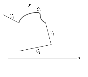
$This is a generic curve in an xy coordinate system with no scales given. It starts with a line in the 2nd quadrant that moves to the right and increasing into the 1st quadrant. This portion is labeled $C_{1}$. The next portion starts picks up and moves slightly to the left and increasing but stays in the 1st quadrant. This portion is labeled $C_{2}$. The third portion is an odd curve that has several dips and curves in it while moving from the 1st quadrant into the 2nd quadrant. This portion is labeled $C_{3}$. The final portion is a line that moves to the left and increases before ending. This portion is labeled $C_{4}$.$

Evaluation of line integrals over piecewise smooth curves is a relatively simple thing to do. All we do is evaluate the line integral over each of the pieces and then add them up. The line integral for some function over the above piecewise curve would be,

\[\int\limits_{C}{{f\left( {x,y} \right)\,ds}} = \int\limits_{{{C_1}}}{{f\left( {x,y} \right)\,ds}} + \int\limits_{{{C_2}}}{{f\left( {x,y} \right)\,ds}} + \int\limits_{{{C_3}}}{{f\left( {x,y} \right)\,ds}} + \int\limits_{{{C_4}}}{{f\left( {x,y} \right)\,ds}}\]

Let’s see an example of this.

Example 2 Evaluate $\displaystyle \int\limits_{C}{{4{x^3}\,ds}}$ where $C$ is the curve shown below.

$This is a curve on an xy coordinate system. The first portion, labeled $C_{1}$ is a horizontal line that starts at (-2,-1) and moves to the right until reaching (0,-1). The second portion, labeled $C_{2}$ is the portion of $y=x^{3}-1$ starting at (-1,0) and moving to the right until reaching (1,0). The final portion, labeled $C_{3}$ is a vertical line that starts at (1,0) and increases until reaching (1,2). There are also arrow heads on each portion indicating the direction the curve is traced out as described above.$

Show Solution

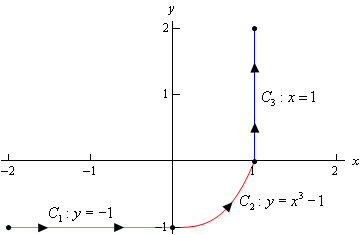
So, first we need to parameterize each of the curves.

\[\begin{align*}& {C_1}\,\,\,:\,\,\,\,x = t,\,\,y = - 1\,,\,\,\,\,\,\,\,\,\,\,\,\, - 2 \le t \le 0\\ & {C_2}\,\,:\,\,\,\,\,x = t,\,\,y = {t^3} - 1,\,\,\,\,\,\,\,\,\,\,0 \le t \le 1\\ & {C_3}\,\,:\,\,\,\,\,x = 1,\,\,\,y = t,\,\,\,\,\,\,\,\,\,\,\,\,\,\,\,\,\,\,\,0 \le t \le 2\end{align*}\]

Now let’s do the line integral over each of these curves.

\[\int\limits_{{{C_1}}}{{4{x^3}\,ds}} = \int_{{\, - 2}}^{{\,0}}{{4{t^3}\sqrt {{{\left( 1 \right)}^2} + {{\left( 0 \right)}^2}} \,dt}} = \int_{{\, - 2}}^{{\,0}}{{4{t^3}\,dt}} = \left. {{t^4}} \right|_{ - 2}^0 = - 16\] \[\begin{align*}\int\limits_{{{C_2}}}{{4{x^3}\,ds}} & = \int_{{\,0}}^{{\,1}}{{4{t^3}\sqrt {{{\left( 1 \right)}^2} + {{\left( {3{t^2}} \right)}^2}} \,dt}}\\ & = \int_{{\,0}}^{{\,1}}{{4{t^3}\sqrt {1 + 9{t^4}} \,dt}}\\ & = \left. {\frac{1}{9}\left( {\frac{2}{3}} \right){{\left( {1 + 9{t^4}} \right)}^{\frac{3}{2}}}} \right|_0^1 = \frac{2}{{27}}\left( {{{10}^{\frac{3}{2}}} - 1} \right) = 2.268\end{align*}\] \[\int\limits_{{{C_3}}}{{4{x^3}\,ds}} = \int_{{\,0}}^{{\,2}}{{4{{\left( 1 \right)}^3}\sqrt {{{\left( 0 \right)}^2} + {{\left( 1 \right)}^2}} \,dt}} = \int_{{\,0}}^{{\,2}}{{4\,dt}} = 8\]

Finally, the line integral that we were asked to compute is,

\[\begin{align*}\int\limits_{C}{{4{x^3}\,ds}} & = \int\limits_{{{C_1}}}{{4{x^3}\,ds}} + \int\limits_{{{C_2}}}{{4{x^3}\,ds}} + \int\limits_{{{C_3}}}{{4{x^3}\,ds}}\\ & = - 16 + 2.268 + 8\\ & = - 5.732\end{align*}\]

Notice that we put direction arrows on the curve in the above example. The direction of motion along a curve may change the value of the line integral as we will see in the next section. Also note that the curve can be thought of a curve that takes us from the point $\left( { - 2, - 1} \right)$ to the point $\left( {1,2} \right)$. Let’s first see what happens to the line integral if we change the path between these two points.

Example 3 Evaluate $\displaystyle\int\limits_{C}{{4{x^3}\,ds}}$ where $C$ is the line segment from $\left( { - 2, - 1} \right)$ to $\left( {1,2} \right)$.

Show Solution

From the parameterization formulas at the start of this section we know that the line segment starting at $\left( { - 2, - 1} \right)$ and ending at $\left( {1,2} \right)$ is given by,

\[\begin{align*}\vec r\left( t \right) & = \left( {1 - t} \right)\left\langle { - 2, - 1} \right\rangle + t\left\langle {1,2} \right\rangle \\ & = \left\langle { - 2 + 3t, - 1 + 3t} \right\rangle \end{align*}\]

for $0 \le t \le 1$. This means that the individual parametric equations are,

\[x = - 2 + 3t\hspace{0.25in}\hspace{0.25in}y = - 1 + 3t\]

Using this path the line integral is,

\[\begin{align*}\int\limits_{C}{{4{x^3}\,ds}} & = \int_{{\,0}}^{{\,1}}{{4{{\left( { - 2 + 3t} \right)}^3}\sqrt {9 + 9} \,dt}}\\ & = 12\sqrt 2 \left( {\frac{1}{{12}}} \right)\left. {{{\left( { - 2 + 3t} \right)}^4}} \right|_0^1\\ & = 12\sqrt 2 \left( { - \frac{5}{4}} \right)\\ & = - 15\sqrt 2 = - 21.213\end{align*}\]

When doing these integrals don’t forget simple Calc I substitutions to avoid having to do things like cubing out a term. Cubing it out is not that difficult, but it is more work than a simple substitution.

So, the previous two examples seem to suggest that if we change the path between two points then the value of the line integral (with respect to arc length) will change. While this will happen fairly regularly we can’t assume that it will always happen. In a later section we will investigate this idea in more detail.

Next, let’s see what happens if we change the direction of a path.

Example 4 Evaluate $\displaystyle \int\limits_{C}{{4{x^3}\,ds}}$ where $C$ is the line segment from $\left( {1,2} \right)$ to $\left( { - 2, - 1} \right)$.

Show Solution

This one isn’t much different, work wise, from the previous example. Here is the parameterization of the curve.

\[\begin{align*}\vec r\left( t \right) & = \left( {1 - t} \right)\left\langle {1,2} \right\rangle + t\left\langle { - 2, - 1} \right\rangle \\ & = \left\langle {1 - 3t,2 - 3t} \right\rangle \end{align*}\]

for $0 \le t \le 1$. Remember that we are switching the direction of the curve and this will also change the parameterization so we can make sure that we start/end at the proper point.

Here is the line integral.

\[\begin{align*}\int\limits_{C}{{4{x^3}\,ds}} & = \int_{{\,0}}^{{\,1}}{{4{{\left( {1 - 3t} \right)}^3}\sqrt {9 + 9} \,dt}}\\ & = 12\sqrt 2 \left( { - \frac{1}{{12}}} \right)\left. {{{\left( {1 - 3t} \right)}^4}} \right|_0^1\\ & = 12\sqrt 2 \left( { - \frac{5}{4}} \right)\\ & = - 15\sqrt 2 = - 21.213\end{align*}\]

So, it looks like when we switch the direction of the curve the line integral (with respect to arc length) will not change. This will always be true for these kinds of line integrals. However, there are other kinds of line integrals in which this won’t be the case. We will see more examples of this in the next couple of sections so don’t get it into your head that changing the direction will never change the value of the line integral.

Before working another example let’s formalize this idea up somewhat. Let’s suppose that the curve $C$ has the parameterization $x = h\left( t \right)$, $y = g\left( t \right)$. Let’s also suppose that the initial point on the curve is $A$ and the final point on the curve is $B$. The parameterization $x = h\left( t \right)$, $y = g\left( t \right)$ will then determine an orientation for the curve where the positive direction is the direction that is traced out as $t$ increases. Finally, let $ - C$ be the curve with the same points as $C$, however in this case the curve has $B$ as the initial point and $A$ as the final point, again $t$ is increasing as we traverse this curve. In other words, given a curve $C$, the curve $ - C$ is the same curve as $C$ except the direction has been reversed.

We then have the following fact about line integrals with respect to arc length.

Fact

\[\int\limits_{C}{{f\left( {x,y} \right)\,ds}} = \int\limits_{{ - C}}{{f\left( {x,y} \right)\,ds}}\]

So, for a line integral with respect to arc length we can change the direction of the curve and not change the value of the integral. This is a useful fact to remember as some line integrals will be easier in one direction than the other.

Now, let’s work another example

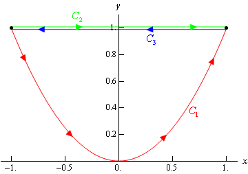
Example 5 Evaluate $\displaystyle \int\limits_{C}{{x\,ds}}$ for each of the following curves.

${C_1}:y = {x^2},\,\,\, - 1 \le x \le 1$
${C_2}$: The line segment from $\left( { - 1,1} \right)$ to $\left( {1,1} \right)$.
${C_3}$: The line segment from $\left( {1,1} \right)$ to $\left( { - 1,1} \right)$.

Show All Solutions Hide All Solutions

Show Discussion

Before working any of these line integrals let’s notice that all of these curves are paths that connect the points $\left( { - 1,1} \right)$ and $\left( {1,1} \right)$. Also notice that ${C_3} = - {C_2}$ and so by the fact above these two should give the same answer.

Here is a sketch of the three curves and note that the curves illustrating ${C_2}$ and ${C_3}$ have been separated a little to show that they are separate curves in some way even though they are the same line.

$This is a curve on an xy coordinate system. It has three distinct curves on it. The first curve, labeled $C_{1}$ is the portion of $y=x^{2}$ moving from (-1,1) to the point (1,1). The second curve, labeled $C_{2}$ is the horizontal line starting at (-1,1) and ending at (1,1). The third curve, labeled $C_{3}$ is the horizontal line starting at (1,1) and ending at (-1,1). Each curve has arrow heads on it indicating the direction of motion as described above.$

a ${C_1}:y = {x^2},\,\,\, - 1 \le x \le 1$ Show Solution

Here is a parameterization for this curve.

\[{C_1}:x = t,\,\,y = {t^2},\,\,\, - 1 \le t \le 1\]

Here is the line integral.

\[\int\limits_{{{C_1}}}{{x\,ds}} = \int_{{\, - 1}}^{{\,1}}{{t\sqrt {1 + 4{t^2}} \,dt}} = \left. {\frac{1}{{12}}{{\left( {1 + 4{t^2}} \right)}^{\frac{3}{2}}}} \right|_{ - 1}^1 = 0\]

b ${C_2}$: The line segment from $\left( { - 1,1} \right)$ to $\left( {1,1} \right)$. Show Solution

There are two parameterizations that we could use here for this curve. The first is to use the formula we used in the previous couple of examples. That parameterization is,

\[\begin{align*}{C_2}:\vec r\left( t \right) & = \left( {1 - t} \right)\left\langle { - 1,1} \right\rangle + t\left\langle {1,1} \right\rangle \\ & \hspace{0.25in}\,\,{\kern 1pt} = \left\langle {2t - 1,1} \right\rangle \end{align*}\]

for $0 \le t \le 1$.

Sometimes we have no choice but to use this parameterization. However, in this case there is a second (probably) easier parameterization. The second one uses the fact that we are really just graphing a portion of the line $y = 1$. Using this the parameterization is,

\[{C_2}:x = t,\,\,y = 1,\,\,\, - 1 \le t \le 1\]

This will be a much easier parameterization to use so we will use this. Here is the line integral for this curve.

\[\int\limits_{{{C_2}}}{{x\,ds}} = \int_{{\, - 1}}^{{\,1}}{{t\sqrt {1 + 0} \,dt}} = \left. {\frac{1}{2}{t^2}} \right|_{ - 1}^1 = 0\]

Note that this time, unlike the line integral we worked with in Examples 2, 3, and 4 we got the same value for the integral despite the fact that the path is different. This will happen on occasion. We should also not expect this integral to be the same for all paths between these two points. At this point all we know is that for these two paths the line integral will have the same value. It is completely possible that there is another path between these two points that will give a different value for the line integral.

c ${C_3}$: The line segment from $\left( {1,1} \right)$ to $\left( { - 1,1} \right)$. Show Solution

Now, according to our fact above we really don’t need to do anything here since we know that ${C_3} = - {C_2}$. The fact tells us that this line integral should be the same as the second part (i.e. zero). However, let’s verify that, plus there is a point we need to make here about the parameterization.

Here is the parameterization for this curve.

\[\begin{align*}{C_3}:\vec r\left( t \right) & = \left( {1 - t} \right)\left\langle {1,1} \right\rangle + t\left\langle { - 1,1} \right\rangle \\ & \hspace{0.25in}\,\,{\kern 1pt} = \left\langle {1 - 2t,1} \right\rangle \end{align*}\]

for $0 \le t \le 1$.

Note that this time we can’t use the second parameterization that we used in part (b) since we need to move from right to left as the parameter increases and the second parameterization used in the previous part will move in the opposite direction.

Here is the line integral for this curve.

\[\int\limits_{{{C_3}}}{{x\,ds}} = \int_{{\,0}}^{{\,1}}{{\left( {1 - 2t} \right)\sqrt {4 + 0} \,dt}} = \left. {2\left( {t - {t^2}} \right)} \right|_0^1 = 0\]

Sure enough we got the same answer as the second part.

To this point in this section we’ve only looked at line integrals over a two-dimensional curve. However, there is no reason to restrict ourselves like that. We can do line integrals over three-dimensional curves as well.

Let’s suppose that the three-dimensional curve $C$ is given by the parameterization,

\[x = x\left( t \right),\,\hspace{0.25in}y = y\left( t \right)\hspace{0.25in}z = z\left( t \right)\hspace{0.25in}a \le t \le b\]

then the line integral is given by,

\[\int\limits_{C}{{f\left( {x,y,z} \right)\,ds}} = \int_{{\,a}}^{{\,b}}{{f\left( {x\left( t \right),y\left( t \right),z\left( t \right)} \right)\sqrt {{{\left( {\frac{{dx}}{{dt}}} \right)}^2} + {{\left( {\frac{{dy}}{{dt}}} \right)}^2} + {{\left( {\frac{{dz}}{{dt}}} \right)}^2}} \,dt}}\]

Note that often when dealing with three-dimensional space the parameterization will be given as a vector function.

\[\vec r\left( t \right) = \left\langle {x\left( t \right),y\left( t \right),z\left( t \right)} \right\rangle \]

Notice that we changed up the notation for the parameterization a little. Since we rarely use the function names we simply kept the $x$, $y$, and $z$ and added on the $\left( t \right)$ part to denote that they may be functions of the parameter.

Also notice that, as with two-dimensional curves, we have,

\[\sqrt {{{\left( {\frac{{dx}}{{dt}}} \right)}^2} + {{\left( {\frac{{dy}}{{dt}}} \right)}^2} + {{\left( {\frac{{dz}}{{dt}}} \right)}^2}} = \left\| {\,\vec r'\left( t \right)} \right\|\]

and the line integral can again be written as,

\[\int\limits_{C}{{f\left( {x,y,z} \right)\,ds}} = \int_{{\,a}}^{{\,b}}{{f\left( {x\left( t \right),y\left( t \right),z\left( t \right)} \right)\,\,\left\| {\vec r'\left( t \right)} \right\|\,dt}}\]

So, outside of the addition of a third parametric equation line integrals in three-dimensional space work the same as those in two-dimensional space. Let’s work a quick example.

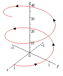
Example 6 Evaluate $\displaystyle \int\limits_{C}{{xyz\,ds}}$ where $C$ is the helix given by, $\vec r\left( t \right) = \left\langle {\cos \left( t \right),\sin \left( t \right),3t} \right\rangle $, $0 \le t \le 4\pi $.

Show Solution

Note that we first saw the vector equation for a helix back in the Vector Functions section. Here is a quick sketch of the helix.

$This is a graph with the standard 3D coordinate system. The positive z-axis is straight up, the positive x-axis moves off to the left and slightly downward and positive y-axis moves off the right and slightly downward. This is the graph of a spiral with radius 1. It starts at the point (1,0,0) and rotates up and around the positive z-axis. It makes two full revolutions before ending at the point (1,0, 12$\pi$).$

Here is the line integral.

\[\begin{align*}\int\limits_{C}{{xyz\,ds}} = \int_{{\,0}}^{{\,4\pi }}{{3t\cos \left( t \right)\sin \left( t \right)\sqrt {{{\sin }^2}t + {{\cos }^2}t + 9} \,dt}}\\ & = \int_{{\,0}}^{{\,4\pi }}{{3t\left( {\frac{1}{2}\sin \left( {2t} \right)} \right)\sqrt {1 + 9} \,dt}}\\ & = \frac{{3\sqrt {10} }}{2}\int_{{\,0}}^{{\,4\pi }}{{t\sin \left( {2t} \right)\,dt}}\\ & = \frac{{3\sqrt {10} }}{2}\left. {\left( {\frac{1}{4}\sin \left( {2t} \right) - \frac{t}{2}\cos \left( {2t} \right)} \right)} \right|_0^{4\pi }\\ & = - 3\sqrt {10} \,\pi \end{align*}\]

You were able to do that integral right? It required integration by parts.

So, as we can see there really isn’t too much difference between two- and three-dimensional line integrals.

Curve	Parametric Equations
\(\begin{array}{c} \displaystyle \frac{{{x^2}}}{{{a^2}}} + \frac{{{y^2}}}{{{b^2}}} = 1 \\ \mbox{(Ellipse)}\end{array}\)	\(\begin{array}{c} \begin{array}{c}\mbox{Counter-Clockwise} \\x = a\cos \left( t \right)\\ y = b\sin \left( t \right)\\ 0 \le t \le 2\pi \end{array}& \begin{array}{c} \mbox{Clockwise} \\x = a\cos \left( t \right)\\ y = - b\sin \left( t \right)\\ 0 \le t \le 2\pi \end{array} \end{array}\)

\(\begin{array}{c}{x^2} + {y^2} = {r^2} \\ \mbox{(Circle)}\end{array}\)	\(\begin{array}{c} \begin{array}{c}\mbox{Counter-Clockwise} \\ x = r\cos \left( t \right)\\ y = r\sin \left( t \right)\\ 0 \le t \le 2\pi \end{array} & \begin{array}{c} \mbox{Clockwise} \\ x = r\cos \left( t \right)\\ y = - r\sin \left( t \right)\\ 0 \le t \le 2\pi \end{array} \end{array}\)

\(y = f\left( x \right)\)	\(\begin{align}x & = t\\ y & = f\left( t \right)\end{align}\)
\(x = g\left( y \right)\)	\(\begin{align}x & = g\left( t \right)\\ y & = t\end{align}\)

\(\begin{array}{l}\mbox{Line Segment From} \\ \left( {{x_0},{y_0},{z_0}} \right) \mbox{ to} \\ \left( {{x_1},{y_1},{z_1}} \right) \end{array}\)	\(\begin{array}{c} \vec r\left( t \right) = \left( {1 - t} \right)\left\langle {{x_0},{y_0},{z_0}} \right\rangle + t\left\langle {{x_1},{y_1},{z_1}} \right\rangle \,\,\,,\,\,0 \le t \le 1 \\ \mbox{or} \\ \begin{array}{l} \begin{aligned} x & = \left( {1 - t} \right){x_0} + t\,{x_1}\\ y & = \left( {1 - t} \right){y_0} + t\,{y_1}\\ z & = \left( {1 - t} \right){z_0} + t\,{z_1} \end{aligned} & , \,\,\,\,\,\, 0 \le t \le 1 \end{array} \end{array}\)