Section 8.2 : Eigenvalues and Eigenfunctions
As we did in the previous section we need to again note that we are only going to give a brief look at the topic of eigenvalues and eigenfunctions for boundary value problems. There are quite a few ideas that we’ll not be looking at here. The intent of this section is simply to give you an idea of the subject and to do enough work to allow us to solve some basic partial differential equations in the next chapter.
Now, before we start talking about the actual subject of this section let’s recall a topic from Linear Algebra that we briefly discussed previously in these notes. For a given square matrix, \(A\), if we could find values of \(\lambda \) for which we could find nonzero solutions, i.e. \(\vec x \ne \vec 0\), to,
\[A\vec x = \lambda \vec x\]then we called \(\lambda \) an eigenvalue of \(A\) and \(\vec x\) was its corresponding eigenvector.
It’s important to recall here that in order for \(\lambda \) to be an eigenvalue then we had to be able to find nonzero solutions to the equation.
So, just what does this have to do with boundary value problems? Well go back to the previous section and take a look at Example 7 and Example 8. In those two examples we solved homogeneous (and that’s important!) BVP’s in the form,
\[\begin{equation}y'' + \lambda y = 0\hspace{0.25in}y\left( 0 \right) = 0\,\,\,\,\,\,\,\,y\left( {2\pi } \right) = 0\label{eq:eq1}\end{equation}\]In Example 7 we had \(\lambda = 4\) and we found nontrivial (i.e. nonzero) solutions to the BVP. In Example 8 we used \(\lambda = 3\) and the only solution was the trivial solution (i.e. \(y\left( t \right) = 0\)). So, this homogeneous BVP (recall this also means the boundary conditions are zero) seems to exhibit similar behavior to the behavior in the matrix equation above. There are values of \(\lambda \) that will give nontrivial solutions to this BVP and values of \(\lambda \) that will only admit the trivial solution.
So, for those values of \(\lambda \) that give nontrivial solutions we’ll call \(\lambda \) an eigenvalue for the BVP and the nontrivial solutions will be called eigenfunctions for the BVP corresponding to the given eigenvalue.
We now know that for the homogeneous BVP given in \(\eqref{eq:eq1}\) \(\lambda = 4\) is an eigenvalue (with eigenfunctions \(y\left( x \right) = {c_2}\sin \left( {2x} \right)\)) and that \(\lambda = 3\) is not an eigenvalue.
Eventually we’ll try to determine if there are any other eigenvalues for \(\eqref{eq:eq1}\), however before we do that let’s comment briefly on why it is so important for the BVP to be homogeneous in this discussion. In Example 2 and Example 3 of the previous section we solved the homogeneous differential equation
\[y'' + 4y = 0\]with two different nonhomogeneous boundary conditions in the form,
\[y\left( 0 \right) = a\hspace{0.25in}y\left( {2\pi } \right) = b\]In these two examples we saw that by simply changing the value of \(a\) and/or \(b\) we were able to get either nontrivial solutions or to force no solution at all. In the discussion of eigenvalues/eigenfunctions we need solutions to exist and the only way to assure this behavior is to require that the boundary conditions also be homogeneous. In other words, we need for the BVP to be homogeneous.
There is one final topic that we need to discuss before we move into the topic of eigenvalues and eigenfunctions and this is more of a notational issue that will help us with some of the work that we’ll need to do.
Let’s suppose that we have a second order differential equation and its characteristic polynomial has two real, distinct roots and that they are in the form
\[{r_1} = \alpha \hspace{0.25in}{r_2} = - \,\alpha \]Then we know that the solution is,
\[y\left( x \right) = {c_1}{{\bf{e}}^{{r_{\,1}}\,x}} + {c_2}{{\bf{e}}^{{r_{\,2}}\,\,x}} = {c_1}{{\bf{e}}^{\alpha \,x}} + {c_2}{{\bf{e}}^{ - \,\,\alpha \,\,x}}\]While there is nothing wrong with this solution let’s do a little rewriting of this. We’ll start by splitting up the terms as follows,
\[\begin{align*}y\left( x \right) & = {c_1}{{\bf{e}}^{\alpha \,x}} + {c_2}{{\bf{e}}^{ - \,\,\alpha \,\,x}}\\ & = \frac{{{c_1}}}{2}{{\bf{e}}^{\alpha \,x}} + \frac{{{c_1}}}{2}{{\bf{e}}^{\alpha \,x}} + \frac{{{c_2}}}{2}{{\bf{e}}^{ - \,\,\alpha \,\,x}} + \frac{{{c_2}}}{2}{{\bf{e}}^{ - \,\,\alpha \,\,x}}\end{align*}\]Now we’ll add/subtract the following terms (note we’re “mixing” the \({c_i}\) and \( \pm \,\alpha \) up in the new terms) to get,
\[y\left( x \right) = \frac{{{c_1}}}{2}{{\bf{e}}^{\alpha \,x}} + \frac{{{c_1}}}{2}{{\bf{e}}^{\alpha \,x}} + \frac{{{c_2}}}{2}{{\bf{e}}^{ - \,\,\alpha \,\,x}} + \frac{{{c_2}}}{2}{{\bf{e}}^{ - \,\,\alpha \,\,x}} + \left( {\frac{{{c_1}}}{2}{{\bf{e}}^{ - \,\,\alpha \,\,x}} - \frac{{{c_1}}}{2}{{\bf{e}}^{ - \,\,\alpha \,\,x}}} \right) + \left( {\frac{{{c_2}}}{2}{{\bf{e}}^{\alpha \,x}} - \frac{{{c_2}}}{2}{{\bf{e}}^{\alpha \,x}}} \right)\]Next, rearrange terms around a little,
\[y\left( x \right) = \frac{1}{2}\left( {{c_1}{{\bf{e}}^{\alpha \,x}} + {c_1}{{\bf{e}}^{ - \,\,\alpha \,\,x}} + {c_2}{{\bf{e}}^{\alpha \,x}} + {c_2}{{\bf{e}}^{ - \,\,\alpha \,\,x}}} \right) + \frac{1}{2}\left( {{c_1}{{\bf{e}}^{\alpha \,x}} - {c_1}{{\bf{e}}^{ - \,\,\alpha \,\,x}} - {c_2}{{\bf{e}}^{\alpha \,x}} + {c_2}{{\bf{e}}^{ - \,\,\alpha \,\,x}}} \right)\]Finally, the quantities in parenthesis factor and we’ll move the location of the fraction as well. Doing this, as well as renaming the new constants we get,
\[\begin{align*}y\left( x \right) & = \left( {{c_1} + {c_2}} \right)\frac{{{{\bf{e}}^{\alpha \,x}} + {{\bf{e}}^{ - \,\,\alpha \,\,x}}}}{2} + \left( {{c_1} - {c_2}} \right)\frac{{{{\bf{e}}^{\alpha \,x}} - {{\bf{e}}^{ - \,\,\alpha \,\,x}}}}{2}\\ & = {{\overline{c}}_1}\frac{{{{\bf{e}}^{\alpha \,x}} + {{\bf{e}}^{ - \,\,\alpha \,\,x}}}}{2} + {{\overline{c}}_2}\frac{{{{\bf{e}}^{\alpha \,x}} - {{\bf{e}}^{ - \,\,\alpha \,\,x}}}}{2}\end{align*}\]All this work probably seems very mysterious and unnecessary. However there really was a reason for it. In fact, you may have already seen the reason, at least in part. The two “new” functions that we have in our solution are in fact two of the hyperbolic functions. In particular,
\[\cosh \left( x \right) = \frac{{{{\bf{e}}^x} + {{\bf{e}}^{ - x}}}}{2}\hspace{0.25in}\sinh \left( x \right) = \frac{{{{\bf{e}}^x} - {{\bf{e}}^{ - x}}}}{2}\]So, another way to write the solution to a second order differential equation whose characteristic polynomial has two real, distinct roots in the form \({r_1} = \alpha ,\,\,{r_2} = - \,\alpha \) is,
\[y\left( x \right) = {c_1}\cosh \left( {\alpha \,x} \right) + {c_2}\sinh \left( {\alpha \,x} \right)\]Having the solution in this form for some (actually most) of the problems we’ll be looking will make our life a lot easier. The hyperbolic functions have some very nice properties that we can (and will) take advantage of.
First, since we’ll be needing them later on, the derivatives are,
\[\frac{d}{{dx}}\left( {\cosh \left( x \right)} \right) = \sinh \left( x \right)\hspace{0.25in}\frac{d}{{dx}}\left( {\sinh \left( x \right)} \right) = \cosh \left( x \right)\]Next let’s take a quick look at the graphs of these functions.
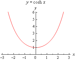
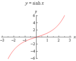
Note that \(\cosh \left( 0 \right) = 1\) and \(\sinh \left( 0 \right) = 0\). Because we’ll often be working with boundary conditions at \(x = 0\) these will be useful evaluations.
Next, and possibly more importantly, let’s notice that \(\cosh \left( x \right) > 0\) for all \(x\) and so the hyperbolic cosine will never be zero. Likewise, we can see that \(\sinh \left( x \right) = 0\) only if \(x = 0\). We will be using both of these facts in some of our work so we shouldn’t forget them.
Okay, now that we’ve got all that out of the way let’s work an example to see how we go about finding eigenvalues/eigenfunctions for a BVP.
We started off this section looking at this BVP and we already know one eigenvalue (\(\lambda = 4\)) and we know one value of \(\lambda \) that is not an eigenvalue (\(\lambda = 3\)). As we go through the work here we need to remember that we will get an eigenvalue for a particular value of \(\lambda \) if we get non-trivial solutions of the BVP for that particular value of \(\lambda \).
In order to know that we’ve found all the eigenvalues we can’t just start randomly trying values of \(\lambda \) to see if we get non-trivial solutions or not. Luckily there is a way to do this that’s not too bad and will give us all the eigenvalues/eigenfunctions. We are going to have to do some cases however. The three cases that we will need to look at are : \(\lambda > 0\), \(\lambda = 0\), and \(\lambda < 0\). Each of these cases gives a specific form of the solution to the BVP to which we can then apply the boundary conditions to see if we’ll get non-trivial solutions or not. So, let’s get started on the cases.
\(\underline {\lambda > 0} \)
In this case the characteristic polynomial we get from the differential equation is,
In this case since we know that \(\lambda > 0\) these roots are complex and we can write them instead as,
\[{r_{1,2}} = \pm \sqrt \lambda \,i\]The general solution to the differential equation is then,
\[y\left( x \right) = {c_1}\cos \left( {\sqrt \lambda \,x} \right) + {c_2}\sin \left( {\sqrt \lambda \,x} \right)\]Applying the first boundary condition gives us,
\[0 = y\left( 0 \right) = {c_1}\]So, taking this into account and applying the second boundary condition we get,
\[0 = y\left( {2\pi } \right) = {c_2}\sin \left( {2\pi \sqrt \lambda } \right)\]This means that we have to have one of the following,
\[{c_2} = 0\hspace{0.25in}{\mbox{or}}\hspace{0.25in}\sin \left( {2\pi \sqrt \lambda } \right) = 0\]However, recall that we want non-trivial solutions and if we have the first possibility we will get the trivial solution for all values of \(\lambda > 0\). Therefore, let’s assume that \({c_2} \ne 0\). This means that we have,
\[\sin \left( {2\pi \sqrt \lambda } \right) = 0\hspace{0.25in} \Rightarrow \hspace{0.25in}2\pi \sqrt \lambda = n\pi \hspace{0.25in}n = 1,2,3, \ldots \]In other words, taking advantage of the fact that we know where sine is zero we can arrive at the second equation. Also note that because we are assuming that \(\lambda > 0\) we know that \(2\pi \sqrt \lambda > 0\)and so \(n\) can only be a positive integer for this case.
Now all we have to do is solve this for \(\lambda \) and we’ll have all the positive eigenvalues for this BVP.
The positive eigenvalues are then,
\[{\lambda _{\,n}} = {\left( {\frac{n}{2}} \right)^2} = \frac{{{n^2}}}{4}\hspace{0.25in}n = 1,2,3, \ldots \]and the eigenfunctions that correspond to these eigenvalues are,
\[{y_n}\left( x \right) = \sin \left( {\frac{{n\,x}}{2}} \right)\hspace{0.25in}n = 1,2,3, \ldots \]Note that we subscripted an \(n\) on the eigenvalues and eigenfunctions to denote the fact that there is one for each of the given values of \(n\). Also note that we dropped the \({c_2}\) on the eigenfunctions. For eigenfunctions we are only interested in the function itself and not the constant in front of it and so we generally drop that.
Let’s now move into the second case.
\(\underline {\lambda = 0} \)
In this case the BVP becomes,
and integrating the differential equation a couple of times gives us the general solution,
\[y\left( x \right) = {c_1} + {c_2}x\]Applying the first boundary condition gives,
\[0 = y\left( 0 \right) = {c_1}\]Applying the second boundary condition as well as the results of the first boundary condition gives,
\[0 = y\left( {2\pi } \right) = 2{c_2}\pi \]Here, unlike the first case, we don’t have a choice on how to make this zero. This will only be zero if \({c_2} = 0\).
Therefore, for this BVP (and that’s important), if we have \(\lambda = 0\) the only solution is the trivial solution and so \(\lambda = 0\) cannot be an eigenvalue for this BVP.
Now let’s look at the final case.
\(\underline {\lambda < 0} \)
In this case the characteristic equation and its roots are the same as in the first case. So, we know that,
However, because we are assuming \(\lambda < 0\) here these are now two real distinct roots and so using our work above for these kinds of real, distinct roots we know that the general solution will be,
\[y\left( x \right) = {c_1}\cosh \left( {\sqrt { - \lambda } \,x} \right) + {c_2}\sinh \left( {\sqrt { - \lambda } \,x} \right)\]Note that we could have used the exponential form of the solution here, but our work will be significantly easier if we use the hyperbolic form of the solution here.
Now, applying the first boundary condition gives,
\[0 = y\left( 0 \right) = {c_1}\cosh \left( 0 \right) + {c_2}\sinh \left( 0 \right) = {c_1}\left( 1 \right) + {c_2}\left( 0 \right) = {c_1}\hspace{0.25in} \Rightarrow \hspace{0.25in}{c_1} = 0\]Applying the second boundary condition gives,
\[0 = y\left( {2\pi } \right) = {c_2}\sinh \left( {2\pi \sqrt { - \lambda } } \right)\]Because we are assuming \(\lambda < 0\) we know that \(2\pi \sqrt { - \lambda } \ne 0\) and so we also know that \(\sinh \left( {2\pi \sqrt { - \lambda } } \right) \ne 0\). Therefore, much like the second case, we must have \({c_2} = 0\).
So, for this BVP (again that’s important), if we have \(\lambda < 0\) we only get the trivial solution and so there are no negative eigenvalues.
In summary then we will have the following eigenvalues/eigenfunctions for this BVP.
\[{\lambda _{\,n}} = \frac{{{n^2}}}{4}\hspace{0.25in}{y_n}\left( x \right) = \sin \left( {\frac{{n\,x}}{2}} \right)\hspace{0.25in}n = 1,2,3, \ldots \]Let’s take a look at another example with slightly different boundary conditions.
Here we are going to work with derivative boundary conditions. The work is pretty much identical to the previous example however so we won’t put in quite as much detail here. We’ll need to go through all three cases just as the previous example so let’s get started on that.
\(\underline {\lambda > 0} \)
The general solution to the differential equation is identical to the previous example and so we have,
Applying the first boundary condition gives us,
\[0 = y'\left( 0 \right) = \sqrt \lambda \,{c_2}\hspace{0.25in} \Rightarrow \hspace{0.25in}{c_2} = 0\]Recall that we are assuming that \(\lambda > 0\) here and so this will only be zero if \({c_2} = 0\). Now, the second boundary condition gives us,
\[0 = y'\left( {2\pi } \right) = - \sqrt \lambda \,{c_1}\sin \left( {2\pi \sqrt \lambda } \right)\]Recall that we don’t want trivial solutions and that \(\lambda > 0\) so we will only get non-trivial solution if we require that,
\[\sin \left( {2\pi \sqrt \lambda } \right) = 0\hspace{0.25in} \Rightarrow \hspace{0.25in}2\pi \sqrt \lambda = n\pi \hspace{0.25in}n = 1,2,3, \ldots \]Solving for \(\lambda \) and we see that we get exactly the same positive eigenvalues for this BVP that we got in the previous example.
\[{\lambda _{\,n}} = {\left( {\frac{n}{2}} \right)^2} = \frac{{{n^2}}}{4}\hspace{0.25in}n = 1,2,3, \ldots \]The eigenfunctions that correspond to these eigenvalues however are,
\[{y_n}\left( x \right) = \cos \left( {\frac{{n\,x}}{2}} \right)\hspace{0.25in}n = 1,2,3, \ldots \]So, for this BVP we get cosines for eigenfunctions corresponding to positive eigenvalues.
Now the second case.
\(\underline {\lambda = 0} \)
The general solution is,
Applying the first boundary condition gives,
\[0 = y'\left( 0 \right) = {c_2}\]Using this the general solution is then,
\[y\left( x \right) = {c_1}\]and note that this will trivially satisfy the second boundary condition,
\[0 = y'\left( {2\pi } \right) = 0\]Therefore, unlike the first example, \(\lambda = 0\) is an eigenvalue for this BVP and the eigenfunctions corresponding to this eigenvalue is,
\[y\left( x \right) = 1\]Again, note that we dropped the arbitrary constant for the eigenfunctions.
Finally let’s take care of the third case.
\(\underline {\lambda < 0} \)
The general solution here is,
Applying the first boundary condition gives,
\[0 = y'\left( 0 \right) = \sqrt { - \lambda } \,{c_1}\sinh \left( 0 \right) + \sqrt { - \lambda } \,{c_2}\cosh \left( 0 \right) = \sqrt { - \lambda } \,{c_2}\hspace{0.25in} \Rightarrow \hspace{0.25in}{c_2} = 0\]Applying the second boundary condition gives,
\[0 = y'\left( {2\pi } \right) = \sqrt { - \lambda } \,{c_1}\sinh \left( {2\pi \sqrt { - \lambda } } \right)\]As with the previous example we again know that \(2\pi \sqrt { - \lambda } \ne 0\) and so \(\sinh \left( {2\pi \sqrt { - \lambda } } \right) \ne 0\). Therefore, we must have \({c_1} = 0\).
So, for this BVP we again have no negative eigenvalues.
In summary then we will have the following eigenvalues/eigenfunctions for this BVP.
\[\begin{align*}{\lambda _{\,n}} & = \frac{{{n^2}}}{4} & {y_n}\left( x \right) & = \cos \left( {\frac{{n\,x}}{2}} \right)\hspace{0.25in}n = 1,2,3, \ldots \\ {\lambda _{\,0}} & = 0 & {y_0}\left( x \right) & = 1\end{align*}\]Notice as well that we can actually combine these if we allow the list of \(n\)’s for the first one to start at zero instead of one. This will often not happen, but when it does we’ll take advantage of it. So the “official” list of eigenvalues/eigenfunctions for this BVP is,
\[{\lambda _{\,n}} = \frac{{{n^2}}}{4}\hspace{0.25in}{y_n}\left( x \right) = \cos \left( {\frac{{n\,x}}{2}} \right)\hspace{0.25in}n = 0,1,2,3, \ldots \]So, in the previous two examples we saw that we generally need to consider different cases for \(\lambda \) as different values will often lead to different general solutions. Do not get too locked into the cases we did here. We will mostly be solving this particular differential equation and so it will be tempting to assume that these are always the cases that we’ll be looking at, but there are BVP’s that will require other/different cases.
Also, as we saw in the two examples sometimes one or more of the cases will not yield any eigenvalues. This will often happen, but again we shouldn’t read anything into the fact that we didn’t have negative eigenvalues for either of these two BVP’s. There are BVP’s that will have negative eigenvalues.
Let’s take a look at another example with a very different set of boundary conditions. These are not the traditional boundary conditions that we’ve been looking at to this point, but we’ll see in the next chapter how these can arise from certain physical problems.
So, in this example we aren’t actually going to specify the solution or its derivative at the boundaries. Instead we’ll simply specify that the solution must be the same at the two boundaries and the derivative of the solution must also be the same at the two boundaries. Also, this type of boundary condition will typically be on an interval of the form [-L,L] instead of [0,L] as we’ve been working on to this point.
As mentioned above these kind of boundary conditions arise very naturally in certain physical problems and we’ll see that in the next chapter.
As with the previous two examples we still have the standard three cases to look at.
\(\underline {\lambda > 0} \)
The general solution for this case is,
Applying the first boundary condition and using the fact that cosine is an even function (i.e.\(\cos \left( { - x} \right) = \cos \left( x \right)\)) and that sine is an odd function (i.e. \(\sin \left( { - x} \right) = - \sin \left( x \right)\)). gives us,
\[\begin{align*}{c_1}\cos \left( { - \pi \sqrt \lambda } \right) + {c_2}\sin \left( { - \pi \sqrt \lambda } \right) & = {c_1}\cos \left( {\pi \sqrt \lambda } \right) + {c_2}\sin \left( {\pi \sqrt \lambda } \right)\\ {c_1}\cos \left( {\pi \sqrt \lambda } \right) - {c_2}\sin \left( {\pi \sqrt \lambda } \right) & = {c_1}\cos \left( {\pi \sqrt \lambda } \right) + {c_2}\sin \left( {\pi \sqrt \lambda } \right)\\ - {c_2}\sin \left( {\pi \sqrt \lambda } \right) & = {c_2}\sin \left( {\pi \sqrt \lambda } \right)\\ 0 & = 2{c_2}\sin \left( {\pi \sqrt \lambda } \right)\end{align*}\]This time, unlike the previous two examples this doesn’t really tell us anything. We could have \(\sin \left( {\pi \sqrt \lambda } \right) = 0\) but it is also completely possible, at this point in the problem anyway, for us to have \({c_2} = 0\) as well.
So, let’s go ahead and apply the second boundary condition and see if we get anything out of that.
\[\begin{align*} - \sqrt \lambda \,{c_1}\sin \left( { - \pi \sqrt \lambda } \right) + \sqrt \lambda \,{c_2}\cos \left( { - \pi \sqrt \lambda } \right) & = - \sqrt \lambda \,{c_1}\sin \left( {\pi \sqrt \lambda } \right) + \sqrt \lambda \,{c_2}\cos \left( {\pi \sqrt \lambda } \right)\\ \sqrt \lambda \,{c_1}\sin \left( {\pi \sqrt \lambda } \right) + \sqrt \lambda \,{c_2}\cos \left( {\pi \sqrt \lambda } \right) & = - \sqrt \lambda \,{c_1}\sin \left( {\pi \sqrt \lambda } \right) + \sqrt \lambda \,{c_2}\cos \left( {\pi \sqrt \lambda } \right)\\ \sqrt \lambda \,{c_1}\sin \left( {\pi \sqrt \lambda } \right) & = - \sqrt \lambda \,{c_1}\sin \left( {\pi \sqrt \lambda } \right)\\ 2\sqrt \lambda \,{c_1}\sin \left( {\pi \sqrt \lambda } \right) & = 0\end{align*}\]So, we get something very similar to what we got after applying the first boundary condition. Since we are assuming that \(\lambda > 0\) this tells us that either \(\sin \left( {\pi \sqrt \lambda } \right) = 0\) or \({c_1} = 0\).
Note however that if \(\sin \left( {\pi \sqrt \lambda } \right) \ne 0\) then we will have to have \({c_1} = {c_2} = 0\) and we’ll get the trivial solution. We therefore need to require that \(\sin \left( {\pi \sqrt \lambda } \right) = 0\) and so just as we’ve done for the previous two examples we can now get the eigenvalues,
\[\pi \sqrt \lambda = n\pi \hspace{0.25in} \Rightarrow \hspace{0.25in}\lambda = {n^2}\,\,\,\,n = 1,2,3, \ldots \]Recalling that \(\lambda > 0\) and we can see that we do need to start the list of possible \(n\)’s at one instead of zero.
So, we now know the eigenvalues for this case, but what about the eigenfunctions. The solution for a given eigenvalue is,
\[y\left( x \right) = {c_1}\cos \left( {n\,x} \right) + {c_2}\sin \left( {n\,x} \right)\]and we’ve got no reason to believe that either of the two constants are zero or non-zero for that matter. In cases like these we get two sets of eigenfunctions, one corresponding to each constant. The two sets of eigenfunctions for this case are,
\[{y_n}\left( x \right) = \cos \left( {n\,x} \right)\hspace{0.25in}{y_n}\left( x \right) = \sin \left( {n\,x} \right)\hspace{0.25in}n = 1,2,3, \ldots \]Now the second case.
\(\underline {\lambda = 0} \)
The general solution is,
Applying the first boundary condition gives,
\[\begin{align*}{c_1} + {c_2}\left( { - \pi } \right) & = {c_1} + {c_2}\left( \pi \right)\\ 2\pi {c_2} & = 0\hspace{0.25in} \Rightarrow \hspace{0.25in}{c_2} = 0\end{align*}\]Using this the general solution is then,
\[y\left( x \right) = {c_1}\]and note that this will trivially satisfy the second boundary condition just as we saw in the second example above. Therefore, we again have \(\lambda = 0\) as an eigenvalue for this BVP and the eigenfunctions corresponding to this eigenvalue is,
\[y\left( x \right) = 1\]Finally let’s take care of the third case.
\(\underline {\lambda < 0} \)
The general solution here is,
Applying the first boundary condition and using the fact that hyperbolic cosine is even and hyperbolic sine is odd gives,
\[\begin{align*}{c_1}\cosh \left( { - \pi \sqrt { - \lambda } } \right) + {c_2}\sinh \left( { - \pi \sqrt { - \lambda } } \right) & = {c_1}\cosh \left( {\pi \sqrt { - \lambda } } \right) + {c_2}\sinh \left( {\pi \sqrt { - \lambda } } \right)\\ - {c_2}\sinh \left( { \pi \sqrt { - \lambda } } \right) & = {c_2}\sinh \left( {\pi \sqrt { - \lambda } } \right)\\ 2{c_2}\sinh \left( {\pi \sqrt { - \lambda } } \right) & = 0\end{align*}\]Now, in this case we are assuming that \(\lambda < 0\) and so we know that \(\pi \sqrt { - \lambda } \ne 0\) which in turn tells us that \(\sinh \left( {\pi \sqrt { - \lambda } } \right) \ne 0\). We therefore must have \({c_2} = 0\).
Let’s now apply the second boundary condition to get,
\[\begin{align*}\sqrt { - \lambda } \,{c_1}\sinh \left( { - \pi \sqrt { - \lambda } } \right) & = \sqrt { - \lambda } \,{c_1}\sinh \left( {\pi \sqrt { - \lambda } } \right)\\ 2\sqrt { - \lambda } \,{c_1}\sinh \left( {\pi \sqrt { - \lambda } } \right) & = 0\hspace{0.25in} \Rightarrow \hspace{0.25in}{c_1} = 0\end{align*}\]By our assumption on \(\lambda \) we again have no choice here but to have \({c_1} = 0\).
Therefore, in this case the only solution is the trivial solution and so, for this BVP we again have no negative eigenvalues.
In summary then we will have the following eigenvalues/eigenfunctions for this BVP.
\[\begin{align*}{\lambda _{\,n}} & = {n^2} & {y_n}\left( x \right) & = \sin \left( {n\,x} \right) & n & = 1,2,3, \ldots \\ {\lambda _{\,n}} & = {n^2} & {y_n}\left( x \right) & = \cos \left( {n\,x} \right) & n & = 1,2,3, \ldots \\ {\lambda _{\,0}} & = 0 & {y_0}\left( x \right) & = 1\end{align*}\]Note that we’ve acknowledged that for \(\lambda > 0\) we had two sets of eigenfunctions by listing them each separately. Also, we can again combine the last two into one set of eigenvalues and eigenfunctions. Doing so gives the following set of eigenvalues and eigenfunctions.
\[\begin{align*}{\lambda _{\,n}} & = {n^2} & {y_n}\left( x \right) & = \sin \left( {n\,x} \right) & n & = 1,2,3, \ldots \\ {\lambda _{\,n}} & = {n^2} & {y_n}\left( x \right) & = \cos \left( {n\,x} \right) & n & = 0,1,2,3, \ldots \end{align*}\]Once again, we’ve got an example with no negative eigenvalues. We can’t stress enough that this is more a function of the differential equation we’re working with than anything and there will be examples in which we may get negative eigenvalues.
Now, to this point we’ve only worked with one differential equation so let’s work an example with a different differential equation just to make sure that we don’t get too locked into this one differential equation.
Before working this example let’s note that we will still be working the vast majority of our examples with the one differential equation we’ve been using to this point. We’re working with this other differential equation just to make sure that we don’t get too locked into using one single differential equation.
This is an Euler differential equation and so we know that we’ll need to find the roots of the following quadratic.
\[r\left( {r - 1} \right) + 3r + \lambda = {r^2} + 2r + \lambda = 0\]The roots to this quadratic are,
\[{r_{1,2}} = \frac{{ - 2 \pm \sqrt {4 - 4\lambda } }}{2} = - 1 \pm \sqrt {1 - \lambda } \]Now, we are going to again have some cases to work with here, however they won’t be the same as the previous examples. The solution will depend on whether or not the roots are real distinct, double or complex and these cases will depend upon the sign/value of \(1 - \lambda \). So, let’s go through the cases.
\(\underline {1 - \lambda < 0,\,\,\lambda > 1} \)
In this case the roots will be complex and we’ll need to write them as follows in order to write down the solution.
By writing the roots in this fashion we know that \(\lambda - 1 > 0\) and so \(\sqrt {\lambda - 1} \) is now a real number, which we need in order to write the following solution,
\[y\left( x \right) = {c_1}{x^{ - 1}}\cos \left( {\ln \left( x \right)\sqrt {\lambda - 1} } \right) + {c_2}{x^{ - 1}}\sin \left( {\ln \left( x \right)\sqrt {\lambda - 1} } \right)\]Applying the first boundary condition gives us,
\[0 = y\left( 1 \right) = {c_1}\cos \left( 0 \right) + {c_2}\sin \left( 0 \right) = {c_1}\hspace{0.25in} \Rightarrow \hspace{0.25in}{c_1} = 0\]The second boundary condition gives us,
\[0 = y\left( 2 \right) = \frac{1}{2}{c_2}\sin \left( {\ln \left( 2 \right)\sqrt {\lambda - 1} } \right)\]In order to avoid the trivial solution for this case we’ll require,
\[\sin \left( {\ln \left( 2 \right)\sqrt {\lambda - 1} } \right) = 0\hspace{0.25in} \Rightarrow \hspace{0.25in}\ln \left( 2 \right)\sqrt {\lambda - 1} = n\pi \hspace{0.25in}n = 1,2,3, \ldots \]This is much more complicated of a condition than we’ve seen to this point, but other than that we do the same thing. So, solving for \(\lambda \) gives us the following set of eigenvalues for this case.
\[{\lambda _{\,n}} = 1 + {\left( {\frac{{n\pi }}{{\ln 2}}} \right)^2}\hspace{0.25in}n = 1,2,3, \ldots \]Note that we need to start the list of \(n\)’s off at one and not zero to make sure that we have \(\lambda > 1\) as we’re assuming for this case.
The eigenfunctions that correspond to these eigenvalues are,
\[{y_n}\left( x \right) = {x^{ - 1}}\sin \left( {\frac{{n\pi }}{{\ln 2}}\ln \left( x \right)} \right)\hspace{0.25in}n = 1,2,3, \ldots \]Now the second case.
\(\underline {1 - \lambda = 0,\,\,\,\lambda = 1} \)
In this case we get a double root of \({r_{\,1,2}} = - 1\) and so the solution is,
Applying the first boundary condition gives,
\[0 = y\left( 1 \right) = {c_1}\]The second boundary condition gives,
\[0 = y\left( 2 \right) = \frac{1}{2}{c_2}\ln \left( 2 \right)\hspace{0.25in} \Rightarrow \hspace{0.25in}{c_2} = 0\]We therefore have only the trivial solution for this case and so \(\lambda = 1\) is not an eigenvalue.
Let’s now take care of the third (and final) case.
\(\underline {1 - \lambda > 0,\,\,\lambda < 1} \)
This case will have two real distinct roots and the solution is,
Applying the first boundary condition gives,
\[0 = y\left( 1 \right) = \,{c_1} + \,{c_2}\hspace{0.25in} \Rightarrow \hspace{0.25in}{c_2} = - {c_1}\]Using this our solution becomes,
\[y\left( x \right) = {c_1}{x^{ - 1 + \sqrt {1 - \lambda } }} - {c_1}{x^{ - 1 - \sqrt {1 - \lambda } }}\]Applying the second boundary condition gives,
\[0 = y\left( 2 \right) = {c_1}{2^{ - 1 + \sqrt {1 - \lambda } }} - {c_1}{2^{ - 1 - \sqrt {1 - \lambda } }} = {c_1}\left( {{2^{ - 1 + \sqrt {1 - \lambda } }} - {2^{ - 1 - \sqrt {1 - \lambda } }}} \right)\]Now, because we know that \(\lambda \ne 1\) for this case the exponents on the two terms in the parenthesis are not the same and so the term in the parenthesis is not the zero. This means that we can only have,
\[{c_1} = {c_2} = 0\]and so in this case we only have the trivial solution and there are no eigenvalues for which \(\lambda < 1\).
The only eigenvalues for this BVP then come from the first case.
So, we’ve now worked an example using a differential equation other than the “standard” one we’ve been using to this point. As we saw in the work however, the basic process was pretty much the same. We determined that there were a number of cases (three here, but it won’t always be three) that gave different solutions. We examined each case to determine if non-trivial solutions were possible and if so found the eigenvalues and eigenfunctions corresponding to that case.
We need to work one last example in this section before we leave this section for some new topics. The four examples that we’ve worked to this point were all fairly simple (with simple being relative of course…), however we don’t want to leave without acknowledging that many eigenvalue/eigenfunctions problems are so easy.
In many examples it is not even possible to get a complete list of all possible eigenvalues for a BVP. Often the equations that we need to solve to get the eigenvalues are difficult if not impossible to solve exactly. So, let’s take a look at one example like this to see what kinds of things can be done to at least get an idea of what the eigenvalues look like in these kinds of cases.
The boundary conditions for this BVP are fairly different from those that we’ve worked with to this point. However, the basic process is the same. So let’s start off with the first case.
\(\underline {\lambda > 0} \)
The general solution to the differential equation is identical to the first few examples and so we have,
Applying the first boundary condition gives us,
\[0 = y\left( 0 \right) = \,{c_1}\hspace{0.25in} \Rightarrow \hspace{0.25in}{c_1} = 0\]The second boundary condition gives us,
\[\begin{align*}0 = y\left( 1 \right) + y'\left( 1 \right) & = \,{c_2}\sin \left( {\sqrt \lambda } \right) + \sqrt \lambda \,{c_2}\cos \left( {\sqrt \lambda } \right)\\ & = \,{c_2}\left( {\sin \left( {\sqrt \lambda } \right) + \sqrt \lambda \,\cos \left( {\sqrt \lambda } \right)} \right)\end{align*}\]So, if we let \({c_2} = 0\) we’ll get the trivial solution and so in order to satisfy this boundary condition we’ll need to require instead that,
\[\begin{align*}0 = \sin \left( {\sqrt \lambda } \right) + \sqrt \lambda \,\cos \left( {\sqrt \lambda } \right)\\ \sin \left( {\sqrt \lambda } \right) & = - \sqrt \lambda \,\cos \left( {\sqrt \lambda } \right)\\ \tan \left( {\sqrt \lambda } \right) & = - \sqrt \lambda \end{align*}\]Now, this equation has solutions but we’ll need to use some numerical techniques in order to get them. In order to see what’s going on here let’s graph \(\tan \left( {\sqrt \lambda } \right)\) and \( - \sqrt \lambda \) on the same graph. Here is that graph and note that the horizontal axis really is values of \(\sqrt \lambda \) as that will make things a little easier to see and relate to values that we’re familiar with.
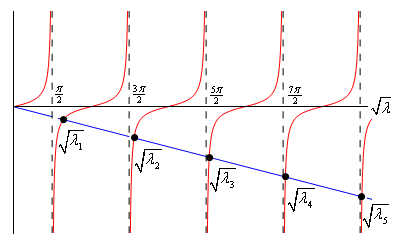
So, eigenvalues for this case will occur where the two curves intersect. We’ve shown the first five on the graph and again what is showing on the graph is really the square root of the actual eigenvalue as we’ve noted.
The interesting thing to note here is that the farther out on the graph the closer the eigenvalues come to the asymptotes of tangent and so we’ll take advantage of that and say that for large enough \(n\) we can approximate the eigenvalues with the (very well known) locations of the asymptotes of tangent.
How large the value of \(n\) is before we start using the approximation will depend on how much accuracy we want, but since we know the location of the asymptotes and as \(n\) increases the accuracy of the approximation will increase so it will be easy enough to check for a given accuracy.
For the purposes of this example we found the first five numerically and then we’ll use the approximation of the remaining eigenvalues. Here are those values/approximations.
\[\begin{align*}\sqrt {{\lambda _{\,1}}} & = 2.0288 & {\lambda _{\,1}} & = 4.1160 & & \left( {2.4674} \right)\\ \sqrt {{\lambda _{\,2}}} & = 4.9132 & {\lambda _{\,2}} & = 24.1395 & & \left( {22.2066} \right)\\ \sqrt {{\lambda _{\,3}}} & = 7.9787 & {\lambda _{\,3}} & = 63.6597 & & \left( {61.6850} \right)\\ \sqrt {{\lambda _{\,4}}} & = 11.0855 & {\lambda _{\,4}} & = 122.8883 & & \left( {120.9027} \right)\\ \sqrt {{\lambda _{\,5}}} & = 14.2074 & {\lambda _{\,5}} & = 201.8502 & & \left( {199.8595} \right)\\ \sqrt {{\lambda _{\,n}}} & \approx \frac{{2n - 1}}{2}\pi & {\lambda _{\,n}} & \approx \frac{{{{\left( {2n - 1} \right)}^2}}}{4}{\pi ^2} & & n = 6,7,8, \ldots \end{align*}\]The number in parenthesis after the first five is the approximate value of the asymptote. As we can see they are a little off, but by the time we get to \(n = 5\) the error in the approximation is 0.9862%. So less than 1% error by the time we get to \(n = 5\) and it will only get better for larger value of \(n\).
The eigenfunctions for this case are,
\[{y_n}\left( x \right) = \sin \left( {\sqrt {{\lambda _{\,n}}} \,x} \right)\hspace{0.25in}n = 1,2,3, \ldots \]where the values of \({\lambda _{\,n}}\) are given above.
So, now that all that work is out of the way let’s take a look at the second case.
\(\underline {\lambda = 0} \)
The general solution is,
Applying the first boundary condition gives,
\[0 = y\left( 0 \right) = {c_1}\]Using this the general solution is then,
\[y\left( x \right) = {c_2}x\]Applying the second boundary condition to this gives,
\[0 = y'\left( 1 \right) + y\left( 1 \right) = {c_2} + {c_2} = 2{c_2}\hspace{0.25in} \Rightarrow \hspace{0.25in}{c_2} = 0\]Therefore, for this case we get only the trivial solution and so \(\lambda = 0\) is not an eigenvalue. Note however that had the second boundary condition been \(y'\left( 1 \right) - y\left( 1 \right) = 0\) then \(\lambda = 0\) would have been an eigenvalue (with eigenfunctions \(y\left( x \right) = x\)) and so again we need to be careful about reading too much into our work here.
Finally let’s take care of the third case.
\(\underline {\lambda < 0} \)
The general solution here is,
Applying the first boundary condition gives,
\[0 = y\left( 0 \right) = {c_1}\cosh \left( 0 \right) + {c_2}\sinh \left( 0 \right) = {c_1}\hspace{0.25in} \Rightarrow \hspace{0.25in}{c_1} = 0\]Using this the general solution becomes,
\[y\left( x \right) = {c_2}\sinh \left( {\sqrt { - \lambda } \,x} \right)\]Applying the second boundary condition to this gives,
\[\begin{align*}0 = y'\left( 1 \right) + y\left( 1 \right) & = \sqrt { - \lambda } {c_2}\cosh \left( {\sqrt { - \lambda } } \right) + {c_2}\sinh \left( {\sqrt { - \lambda } } \right)\\ & = {c_2}\left( {\sqrt { - \lambda } \cosh \left( {\sqrt { - \lambda } } \right) + \sinh \left( {\sqrt { - \lambda } } \right)} \right)\end{align*}\]Now, by assumption we know that \(\lambda < 0\) and so \(\sqrt { - \lambda } > 0\). This in turn tells us that \(\sinh \left( {\sqrt { - \lambda } } \right) > 0\) and we know that \(\cosh \left( x \right) > 0\) for all \(x\). Therefore,
\[\sqrt { - \lambda } \cosh \left( {\sqrt { - \lambda } } \right) + \sinh \left( {\sqrt { - \lambda } } \right) \ne 0\]and so we must have \({c_2} = 0\) and once again in this third case we get the trivial solution and so this BVP will have no negative eigenvalues.
In summary the only eigenvalues for this BVP come from assuming that \(\lambda > 0\) and they are given above.
So, we’ve worked several eigenvalue/eigenfunctions examples in this section. Before leaving this section we do need to note once again that there are a vast variety of different problems that we can work here and we’ve really only shown a bare handful of examples and so please do not walk away from this section believing that we’ve shown you everything.
The whole purpose of this section is to prepare us for the types of problems that we’ll be seeing in the next chapter. Also, in the next chapter we will again be restricting ourselves down to some pretty basic and simple problems in order to illustrate one of the more common methods for solving partial differential equations.