Section 5.9 : Repeated Eigenvalues
This is the final case that we need to take a look at. In this section we are going to look at solutions to the system,
\[\vec x' = A\vec x\]where the eigenvalues are repeated eigenvalues. Since we are going to be working with systems in which \(A\) is a \(2 \times 2\) matrix we will make that assumption from the start. So, the system will have a double eigenvalue, \(\lambda \).
This presents us with a problem. We want two linearly independent solutions so that we can form a general solution. However, with a double eigenvalue we will have only one,
\[{\vec x_1} = \vec \eta {{\bf{e}}^{\lambda t}}\]So, we need to come up with a second solution. Recall that when we looked at the double root case with the second order differential equations we ran into a similar problem. In that section we simply added a \(t\) to the solution and were able to get a second solution. Let’s see if the same thing will work in this case as well. We’ll see if
\[\vec x = t\,{{\bf{e}}^{\lambda t}}\vec \eta \]will also be a solution.
To check all we need to do is plug into the system. Don’t forget to product rule the proposed solution when you differentiate!
\[\vec \eta {{\bf{e}}^{\lambda t}} + \lambda \vec \eta t{{\bf{e}}^{\lambda t}} = A\vec \eta t{{\bf{e}}^{\lambda t}}\]Now, we got two functions here on the left side, an exponential by itself and an exponential times a \(t\). So, in order for our guess to be a solution we will need to require,
\[\begin{align*}A\vec \eta & = \lambda \vec \eta \hspace{0.25in} \Rightarrow \hspace{0.25in}\left( {A - \lambda I} \right)\vec \eta = \vec 0\\ \vec \eta & = \vec 0\end{align*}\]The first requirement isn’t a problem since this just says that \(\lambda \) is an eigenvalue and it’s eigenvector is \(\vec \eta \). We already knew this however so there’s nothing new there. The second however is a problem. Since \(\vec \eta \)is an eigenvector we know that it can’t be zero, yet in order to satisfy the second condition it would have to be.
So, our guess was incorrect. The problem seems to be that there is a lone term with just an exponential in it so let’s see if we can’t fix up our guess to correct that. Let’s try the following guess.
\[\vec x = t\,{{\bf{e}}^{\lambda t}}\vec \eta + {{\bf{e}}^{\lambda t}}\vec \rho \]where \(\vec \rho \) is an unknown vector that we’ll need to determine.
As with the first guess let’s plug this into the system and see what we get.
\[\begin{align*}\vec \eta {{\bf{e}}^{\lambda t}} + \lambda \vec \eta t{{\bf{e}}^{\lambda t}} + \lambda \vec \rho {{\bf{e}}^{\lambda t}} & = A\left( {\vec \eta t{{\bf{e}}^{\lambda t}} + \vec \rho {{\bf{e}}^{\lambda t}}} \right)\\ \left( {\vec \eta + \lambda \vec \rho } \right){{\bf{e}}^{\lambda t}} + \lambda \vec \eta t{{\bf{e}}^{\lambda t}} & = A\vec \eta t{{\bf{e}}^{\lambda t}} + A\vec \rho {{\bf{e}}^{\lambda t}}\end{align*}\]Now set coefficients equal again,
\[\begin{align*}\lambda \vec \eta & = A\vec \eta & \Rightarrow \hspace{0.25in}\left( {A - \lambda I} \right)\vec \eta & = \vec 0\\ \vec \eta + \lambda \vec \rho & = A\vec \rho & \Rightarrow \hspace{0.25in}\left( {A - \lambda I} \right)\vec \rho & = \vec \eta \end{align*}\]As with our first guess the first equation tells us nothing that we didn’t already know. This time the second equation is not a problem. All the second equation tells us is that \(\vec \rho \) must be a solution to this equation.
It looks like our second guess worked. Therefore,
\[{\vec x_2} = t\,{{\bf{e}}^{\lambda t}}\vec \eta + {{\bf{e}}^{\lambda t}}\vec \rho \]will be a solution to the system provided \(\vec \rho \) is a solution to
\[\left( {A - \lambda I} \right)\vec \rho = \vec \eta \]Also, this solution and the first solution are linearly independent and so they form a fundamental set of solutions and so the general solution in the double eigenvalue case is,
\[\vec x = {c_1}\,{{\bf{e}}^{\lambda t}}\vec \eta + {c_2}\left( {t\,{{\bf{e}}^{\lambda t}}\vec \eta + {{\bf{e}}^{\lambda t}}\vec \rho } \right)\]Let’s work an example.
First find the eigenvalues for the system.
\[\begin{align*}\det \left( {A - \lambda I} \right) & = \left| {\begin{array}{*{20}{c}}{7 - \lambda }&1\\{ - 4}&{3 - \lambda }\end{array}} \right|\\ & = {\lambda ^2} - 10\lambda + 25\\ & = {\left( {\lambda - 5} \right)^2}\hspace{0.25in} \Rightarrow \hspace{0.25in}{\lambda _{1,2}} = 5\end{align*}\]So, we got a double eigenvalue. Of course, that shouldn’t be too surprising given the section that we’re in. Let’s find the eigenvector for this eigenvalue.
\[\left( {\begin{array}{*{20}{c}}2&1\\{ - 4}&{ - 2}\end{array}} \right)\left( {\begin{array}{*{20}{c}}{{\eta _1}}\\{{\eta _2}}\end{array}} \right) = \left( {\begin{array}{*{20}{c}}0\\0\end{array}} \right)\hspace{0.25in} \Rightarrow \,\hspace{0.25in}2{\eta _1} + {\eta _2} = 0\hspace{0.25in}{\eta _2} = - 2{\eta _1}\]The eigenvector is then,
\[\begin{align*}\vec \eta & = \left( {\begin{array}{*{20}{c}}{{\eta _1}}\\{ - 2{\eta _1}}\end{array}} \right) & \hspace{0.25in}{\eta _1} & \ne 0\\ {{\vec \eta }^{\left( 1 \right)}} & = \left( {\begin{array}{*{20}{c}}1\\{ - 2}\end{array}} \right) & \hspace{0.25in}{\eta _1} & = 1\end{align*}\]The next step is find \(\vec \rho \). To do this we’ll need to solve,
\[\left( {\begin{array}{*{20}{c}}2&1\\{ - 4}&{ - 2}\end{array}} \right)\left( {\begin{array}{*{20}{c}}{{\rho _1}}\\{{\rho _2}}\end{array}} \right) = \left( {\begin{array}{*{20}{c}}1\\{ - 2}\end{array}} \right)\hspace{0.25in} \Rightarrow \,\hspace{0.25in}2{\rho _1} + {\rho _2} = 1\hspace{0.25in}{\rho _2} = 1 - 2{\rho _1}\]Note that this is almost identical to the system that we solve to find the eigenvalue. The only difference is the right hand side. The most general possible \(\vec \rho \) is
\[\vec \rho = \left( {\begin{array}{*{20}{c}}{{\rho _1}}\\{1 - 2{\rho _1}}\end{array}} \right)\hspace{0.25in} \Rightarrow \hspace{0.25in}\vec \rho = \left( {\begin{array}{*{20}{c}}0\\1\end{array}} \right)\hspace{0.25in}{\mbox{if }}{\rho _1} = 0\]In this case, unlike the eigenvector system we can choose the constant to be anything we want, so we might as well pick it to make our life easier. This usually means picking it to be zero.
We can now write down the general solution to the system.
\[\vec x\left( t \right) = {c_1}{{\bf{e}}^{5t}}\left( {\begin{array}{*{20}{c}}1\\{ - 2}\end{array}} \right) + {c_2}\left( {{{\bf{e}}^{5t}}t\left( {\begin{array}{*{20}{c}}1\\{ - 2}\end{array}} \right) + {{\bf{e}}^{5t}}\left( {\begin{array}{*{20}{c}}0\\1\end{array}} \right)} \right)\]Applying the initial condition to find the constants gives us,
\[\left( {\begin{array}{*{20}{c}}2\\{ - 5}\end{array}} \right) = \vec x\left( 0 \right) = {c_1}\left( {\begin{array}{*{20}{c}}1\\{ - 2}\end{array}} \right) + {c_2}\left( {\begin{array}{*{20}{c}}0\\1\end{array}} \right)\] \[\left. {\begin{array}{*{20}{r}}{{c_1} = 2}\\{ - 2{c_1} + {c_2} = - 5}\end{array}} \right\}\hspace{0.25in} \Rightarrow \hspace{0.25in}{c_1} = 2,\,\,\,{c_2} = - 1\]The actual solution is then,
\[\begin{align*}\vec x\left( t \right) & = 2{{\bf{e}}^{5t}}\left( {\begin{array}{*{20}{c}}1\\{ - 2}\end{array}} \right) - \left( {t{{\bf{e}}^{5t}}\left( {\begin{array}{*{20}{c}}1\\{ - 2}\end{array}} \right) + {{\bf{e}}^{5t}}\left( {\begin{array}{*{20}{c}}0\\1\end{array}} \right)} \right)\\ & = {{\bf{e}}^{5t}}\left( {\begin{array}{*{20}{c}}2\\{ - 4}\end{array}} \right) - {{\bf{e}}^{5t}}t\left( {\begin{array}{*{20}{c}}1\\{ - 2}\end{array}} \right) - {{\bf{e}}^{5t}}\left( {\begin{array}{*{20}{c}}0\\1\end{array}} \right)\\ & = {{\bf{e}}^{5t}}\left( {\begin{array}{*{20}{c}}2\\{ - 5}\end{array}} \right) - {{\bf{e}}^{5t}}t\left( {\begin{array}{*{20}{c}}1\\{ - 2}\end{array}} \right)\end{align*}\]Note that we did a little combining here to simplify the solution up a little.
So, the next example will be to sketch the phase portrait for this system.
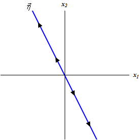
These will start in the same way that real, distinct eigenvalue phase portraits start. We’ll first sketch in a trajectory that is parallel to the eigenvector and note that since the eigenvalue is positive the trajectory will be moving away from the origin.
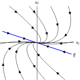
Now, it will be easier to explain the remainder of the phase portrait if we actually have one in front of us. So here is the full phase portrait with some more trajectories sketched in.
Trajectories in these cases always emerge from (or move into) the origin in a direction that is parallel to the eigenvector. Likewise, they will start in one direction before turning around and moving off into the other direction. The directions in which they move are opposite depending on which side of the trajectory corresponding to the eigenvector we are on. Also, as the trajectories move away from the origin it should start becoming parallel to the trajectory corresponding to the eigenvector.
So, how do we determine the direction? We can do the same thing that we did in the complex case. We’ll plug in \(\left( {1,0} \right)\) into the system and see which direction the trajectories are moving at that point. Since this point is directly to the right of the origin the trajectory at that point must have already turned around and so this will give the direction that it will traveling after turning around.
Doing that for this problem to check our phase portrait gives,
\[\left( {\begin{array}{*{20}{c}}7&1\\{ - 4}&3\end{array}} \right)\left( {\begin{array}{*{20}{c}}1\\0\end{array}} \right) = \left( {\begin{array}{*{20}{c}}7\\{ - 4}\end{array}} \right)\]This vector will point down into the fourth quadrant and so the trajectory must be moving into the fourth quadrant as well. This does match up with our phase portrait.
In these cases, the equilibrium is called a node and is unstable in this case. Note that sometimes you will hear nodes for the repeated eigenvalue case called degenerate nodes or improper nodes.
Let’s work one more example.
First the eigenvalue for the system.
\[\begin{align*}\det \left( {A - \lambda I} \right) & = \left| {\begin{array}{*{20}{c}}{ - 1 - \lambda }&{\frac{3}{2}}\\{ - \frac{1}{6}}&{ - 2 - \lambda }\end{array}} \right|\\ & = {\lambda ^2} + 3\lambda + \frac{9}{4}\\ & = {\left( {\lambda + \frac{3}{2}} \right)^2}\hspace{0.25in} \Rightarrow \hspace{0.25in}{\lambda _{1,2}} = - \frac{3}{2}\end{align*}\]Now let’s get the eigenvector.
\[\left( {\begin{array}{*{20}{c}}{\frac{1}{2}}&{\frac{3}{2}}\\{ - \frac{1}{6}}&{ - \frac{1}{2}}\end{array}} \right)\left( {\begin{array}{*{20}{c}}{{\eta _1}}\\{{\eta _2}}\end{array}} \right) = \left( {\begin{array}{*{20}{c}}0\\0\end{array}} \right)\hspace{0.25in} \Rightarrow \,\hspace{0.25in}\frac{1}{2}{\eta _1} + \frac{3}{2}{\eta _2} = 0\,\,\,\,\,\,\,\,\,{\eta _1} = - 3{\eta _2}\] \[\begin{align*}\vec \eta & = \left( {\begin{array}{*{20}{c}}{ - 3{\eta _2}}\\{{\eta _2}}\end{array}} \right) & \hspace{0.25in}{\eta _2} & \ne 0\\ {{\vec \eta }^{\left( 1 \right)}} & = \left( {\begin{array}{*{20}{c}}{ - 3}\\1\end{array}} \right) & \hspace{0.25in}{\eta _2} & = 1\end{align*}\]Now find \(\vec \rho \),
\[\left( {\begin{array}{*{20}{c}}{\frac{1}{2}}&{\frac{3}{2}}\\{ - \frac{1}{6}}&{ - \frac{1}{2}}\end{array}} \right)\left( {\begin{array}{*{20}{c}}{{\rho _1}}\\{{\rho _2}}\end{array}} \right) = \left( {\begin{array}{*{20}{c}}{ - 3}\\1\end{array}} \right)\hspace{0.25in} \Rightarrow \,\hspace{0.25in}\frac{1}{2}{\rho _1} + \frac{3}{2}{\rho _2} = - 3\,\,\,\,\,\,\,\,\,{\rho _1} = - 6 - 3{\rho _2}\] \[\vec \rho = \left( {\begin{array}{*{20}{c}}{ - 6 - 3{\rho _2}}\\{{\rho _2}}\end{array}} \right)\hspace{0.25in} \Rightarrow \hspace{0.25in}\vec \rho = \left( {\begin{array}{*{20}{c}}{ - 6}\\0\end{array}} \right)\hspace{0.25in}{\mbox{if }}{\rho _2} = 0\]The general solution for the system is then,
\[\vec x\left( t \right) = {c_1}{{\bf{e}}^{ - \frac{{3t}}{2}}}\left( {\begin{array}{*{20}{c}}{ - 3}\\1\end{array}} \right) + {c_2}\left( {t{{\bf{e}}^{ - \frac{{3t}}{2}}}\left( {\begin{array}{*{20}{c}}{ - 3}\\1\end{array}} \right) + {{\bf{e}}^{ - \frac{{3t}}{2}}}\left( {\begin{array}{*{20}{c}}{ - 6}\\0\end{array}} \right)} \right)\]Applying the initial condition gives,
\[\left( {\begin{array}{*{20}{c}}1\\0\end{array}} \right) = \vec x\left( 2 \right) = {c_1}{{\bf{e}}^{ - 3}}\left( {\begin{array}{*{20}{c}}{ - 3}\\1\end{array}} \right) + {c_2}\left( {2{{\bf{e}}^{ - 3}}\left( {\begin{array}{*{20}{c}}{ - 3}\\1\end{array}} \right) + {{\bf{e}}^{ - 3}}\left( {\begin{array}{*{20}{c}}{ - 6}\\0\end{array}} \right)} \right)\]Note that we didn’t use \(t=0\) this time! We now need to solve the following system,
\[\left. {\begin{array}{*{20}{r}}{ - 3{{\bf{e}}^{ - 3}}{c_1} - 12{{\bf{e}}^{ - 3}}{c_2} = 1}\\{{{\bf{e}}^{ - 3}}{c_1} + 2{{\bf{e}}^{ - 3}}{c_2} = 0}\end{array}} \right\}\hspace{0.25in} \Rightarrow \hspace{0.25in}{c_1} = \frac{{{{\bf{e}}^3}}}{3},\,\,\,{c_2} = - \frac{{{{\bf{e}}^3}}}{6}\]The actual solution is then,
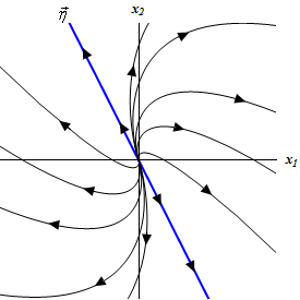
\[\begin{align*}\vec x\left( t \right) &= \frac{{{{\bf{e}}^3}}}{3}{{\bf{e}}^{ - \frac{{3t}}{2}}}\left( {\begin{array}{*{20}{c}}{ - 3}\\1\end{array}} \right) - \frac{{{{\bf{e}}^3}}}{6}\left( {t{{\bf{e}}^{ - \frac{{3t}}{2}}}\left( {\begin{array}{*{20}{c}}{ - 3}\\1\end{array}} \right) + {{\bf{e}}^{ - \frac{{3t}}{2}}}\left( {\begin{array}{*{20}{c}}{ - 6}\\0\end{array}} \right)} \right)\\ & = {{\bf{e}}^{ - \frac{{3t}}{2} + 3}}\left( {\begin{array}{*{20}{c}}0\\{\frac{1}{3}}\end{array}} \right) + t{{\bf{e}}^{ - \frac{{3t}}{2} + 3}}\left( {\begin{array}{*{20}{c}}{\frac{1}{2}}\\{ - \frac{1}{6}}\end{array}} \right)\end{align*}\]And just to be consistent with all the other problems that we’ve done let’s sketch the phase portrait.
Let’s first notice that since the eigenvalue is negative in this case the trajectories should all move in towards the origin. Let’s check the direction of the trajectories at \(\left( {1,0} \right)\).
\[\left( {\begin{array}{*{20}{c}}{ - 1}&{\frac{3}{2}}\\{ - \frac{1}{6}}&{ - 2}\end{array}} \right)\left( {\begin{array}{*{20}{c}}1\\0\end{array}} \right) = \left( {\begin{array}{*{20}{c}}{ - 1}\\{ - \frac{1}{6}}\end{array}} \right)\]So, it looks like the trajectories should be pointing into the third quadrant at \(\left( {1,0} \right)\). This gives the following phase portrait.