Section 2.1 : Tangent Lines and Rates of Change
In this section we are going to take a look at two fairly important problems in the study of calculus. There are two reasons for looking at these problems now.
First, both of these problems will lead us into the study of limits, which is the topic of this chapter after all. Looking at these problems here will allow us to start to understand just what a limit is and what it can tell us about a function.
Secondly, the rate of change problem that we’re going to be looking at is one of the most important concepts that we’ll encounter in the second chapter of this course. In fact, it’s probably one of the most important concepts that we’ll encounter in the whole course. So, looking at it now will get us to start thinking about it from the very beginning.
Tangent Lines
The first problem that we’re going to take a look at is the tangent line problem. Before getting into this problem it would probably be best to define a tangent line.
A tangent line to the function \(f(x)\) at the point \(x = a\) is a line that just touches the graph of the function at the point in question and is “parallel” (in some way) to the graph at that point. Take a look at the graph below.
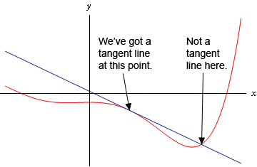
In this graph the line is a tangent line at the indicated point because it just touches the graph at that point and is also “parallel” to the graph at that point. Likewise, at the second point shown, the line does just touch the graph at that point, but it is not “parallel” to the graph at that point and so it’s not a tangent line to the graph at that point.
At the second point shown (the point where the line isn’t a tangent line) we will sometimes call the line a secant line.
We’ve used the word parallel a couple of times now and we should probably be a little careful with it. In general, we will think of a line and a graph as being parallel at a point if they are both moving in the same direction at that point. So, in the first point above the graph and the line are moving in the same direction and so we will say they are parallel at that point. At the second point, on the other hand, the line and the graph are not moving in the same direction so they aren’t parallel at that point.
Okay, now that we’ve gotten the definition of a tangent line out of the way let’s move on to the tangent line problem. That’s probably best done with an example.
We know from algebra that to find the equation of a line we need either two points on the line or a single point on the line and the slope of the line. Since we know that we are after a tangent line we do have a point that is on the line. The tangent line and the graph of the function must touch at \(x\) = 1 so the point \(\left( {1,f\left( 1 \right)} \right) = \left( {1,13} \right)\) must be on the line.
Now we reach the problem. This is all that we know about the tangent line. In order to find the tangent line we need either a second point or the slope of the tangent line. Since the only reason for needing a second point is to allow us to find the slope of the tangent line let’s just concentrate on seeing if we can determine the slope of the tangent line.
At this point in time all that we’re going to be able to do is to get an estimate for the slope of the tangent line, but if we do it correctly we should be able to get an estimate that is in fact the actual slope of the tangent line. We’ll do this by starting with the point that we’re after, let’s call it \(P = \left( {1,13} \right)\). We will then pick another point that lies on the graph of the function, let’s call that point \(Q = \left( {x,f\left( x \right)} \right)\).
For the sake of argument let’s take \(x = 2\) and so the second point will be \(Q = \left( {2,7} \right)\). Below is a graph of the function, the tangent line and the secant line that connects \(P\) and \(Q\).
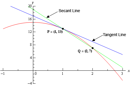
We can see from this graph that the secant and tangent lines are somewhat similar and so the slope of the secant line should be somewhat close to the actual slope of the tangent line. So, as an estimate of the slope of the tangent line we can use the slope of the secant line, let’s call it \({m_{PQ}}\), which is,
\[{m_{PQ}} = \frac{{f\left( 2 \right) - f\left( 1 \right)}}{{2 - 1}} = \frac{{7 - 13}}{1} = - 6\]Now, if we weren’t too interested in accuracy we could say this is good enough and use this as an estimate of the slope of the tangent line. However, we would like an estimate that is at least somewhat close the actual value. So, to get a better estimate we can take an \(x\) that is closer to \(x = 1\) and redo the work above to get a new estimate on the slope. We could then take a third value of \(x\) even closer yet and get an even better estimate.
In other words, as we take \(Q\) closer and closer to \(P\) the slope of the secant line connecting \(Q\) and \(P\) should be getting closer and closer to the slope of the tangent line. If you are viewing this on the web, the image below shows this process.
As you can see (animation won't work on all pdf viewers unfortunately) as we moved \(Q\) in closer and closer to \(P\) the secant lines does start to look more and more like the tangent line and so the approximate slopes (i.e. the slopes of the secant lines) are getting closer and closer to the exact slope. Also, do not worry about how I got the exact or approximate slopes. We’ll be computing the approximate slopes shortly and we’ll be able to compute the exact slope in a few sections.
In this figure we only looked at \(Q\)’s that were to the right of \(P\), but we could have just as easily used \(Q\)’s that were to the left of \(P\) and we would have received the same results. In fact, we should always take a look at \(Q\)’s that are on both sides of \(P\). In this case the same thing is happening on both sides of \(P\). However, we will eventually see that doesn’t have to happen. Therefore, we should always take a look at what is happening on both sides of the point in question when doing this kind of process.
So, let’s see if we can come up with the approximate slopes we showed above, and hence an estimation of the slope of the tangent line. In order to simplify the process a little let’s get a formula for the slope of the line between \(P\) and \(Q\), \({m_{PQ}}\), that will work for any \(x\) that we choose to work with. We can get a formula by finding the slope between \(P\) and \(Q\) using the “general” form of \(Q = \left( {x,f\left( x \right)} \right)\).
\[{m_{PQ}} = \frac{{f\left( x \right) - f\left( 1 \right)}}{{x - 1}} = \frac{{15 - 2{x^2} - 13}}{{x - 1}} = \frac{{2 - 2{x^2}}}{{x - 1}}\]Now, let’s pick some values of \(x\) getting closer and closer to \(x = 1\), plug in and get some slopes.
| \(x\) | \({m_{PQ}}\) | \(x\) | \({m_{PQ}}\) |
|---|---|---|---|
| 2 | -6 | 0 | -2 |
| 1.5 | -5 | 0.5 | -3 |
| 1.1 | -4.2 | 0.9 | -3.8 |
| 1.01 | -4.02 | 0.99 | -3.98 |
| 1.001 | -4.002 | 0.999 | -3.998 |
| 1.0001 | -4.0002 | 0.9999 | -3.9998 |
So, if we take \(x\)’s to the right of 1 and move them in very close to 1 it appears that the slope of the secant lines appears to be approaching -4. Likewise, if we take \(x\)’s to the left of 1 and move them in very close to 1 the slope of the secant lines again appears to be approaching -4.
Based on this evidence it seems that the slopes of the secant lines are approaching -4 as we move in towards \(x = 1\), so we will estimate that the slope of the tangent line is also -4. As noted above, this is the correct value and we will be able to prove this eventually.
Now, the equation of the line that goes through \[\left( {a,f\left( a \right)} \right)\] is given by
\[y = f\left( a \right) + m\left( {x - a} \right)\]Therefore, the equation of the tangent line to \(f\left( x \right) = 15 - 2{x^2}\) at \(x=1\) is
\[y = 13 - 4\left( {x - 1} \right) = - 4x + 17\]There are a couple of important points to note about our work above. First, we looked at points that were on both sides of \(x = 1\). In this kind of process it is important to never assume that what is happening on one side of a point will also be happening on the other side as well. We should always look at what is happening on both sides of the point. In this example we could sketch a graph and from that guess that what is happening on one side will also be happening on the other, but we will usually not have the graphs in front of us or be able to easily get them.
Next, notice that when we say we’re going to move in close to the point in question we do mean that we’re going to move in very close and we also used more than just a couple of points. We should never try to determine a trend based on a couple of points that aren’t really all that close to the point in question.
The next thing to notice is really a warning more than anything. The values of \({m_{PQ}}\) in this example were fairly “nice” and it was pretty clear what value they were approaching after a couple of computations. In most cases this will not be the case. Most values will be far “messier” and you’ll often need quite a few computations to be able to get an estimate. You should always use at least four points, on each side to get the estimate. Two points is never sufficient to get a good estimate and three points will also often not be sufficient to get a good estimate. Generally, you keeping picking points closer and closer to the point you are looking at until the change in the value between two successive points is getting very small.
Last, we were after something that was happening at \(x = 1\) and we couldn’t actually plug \(x = 1\) into our formula for the slope. Despite this limitation we were able to determine some information about what was happening at \(x = 1\) simply by looking at what was happening around \(x = 1\). This is more important than you might at first realize and we will be discussing this point in detail in later sections.
Before moving on let’s do a quick review of just what we did in the above example. We wanted the tangent line to \(f\left( x \right)\) at a point \(x = a\). First, we know that the point \(P = \left( {a,f\left( a \right)} \right)\) will be on the tangent line. Next, we’ll take a second point that is on the graph of the function, call it \(Q = \left( {x,f\left( x \right)} \right)\) and compute the slope of the line connecting \(P\) and \(Q\) as follows,
\[{m_{PQ}} = \frac{{f\left( x \right) - f\left( a \right)}}{{x - a}}\]We then take values of \(x\) that get closer and closer to \(x = a\) (making sure to look at \(x\)’s on both sides of \(x = a\) and use this list of values to estimate the slope of the tangent line, \(m\).
The tangent line will then be,
\[y = f\left( a \right) + m\left( {x - a} \right)\]Rates of Change
The next problem that we need to look at is the rate of change problem. As mentioned earlier, this will turn out to be one of the most important concepts that we will look at throughout this course.
Here we are going to consider a function, \(f\left( x \right)\), that represents some quantity that varies as \(x\) varies. For instance, maybe \(f\left( x \right)\) represents the amount of water in a holding tank after \(x\) minutes. Or maybe \(f\left( x \right)\) is the distance traveled by a car after \(x\) hours. In both of these example we used \(x\) to represent time. Of course \(x\) doesn’t have to represent time, but it makes for examples that are easy to visualize.
What we want to do here is determine just how fast \(f\left( x \right)\) is changing at some point, say \(x = a\). This is called the instantaneous rate of change or sometimes just rate of change of \(f\left( x \right)\) at \(x = a\).
As with the tangent line problem all that we’re going to be able to do at this point is to estimate the rate of change. So, let’s continue with the examples above and think of \(f\left( x \right)\) as something that is changing in time and \(x\) being the time measurement. Again, \(x\) doesn’t have to represent time but it will make the explanation a little easier. While we can’t compute the instantaneous rate of change at this point we can find the average rate of change.
To compute the average rate of change of \(f\left( x \right)\) at \(x = a\) all we need to do is to choose another point, say \(x\), and then the average rate of change will be,
\[\begin{align*}A.R.C. & = \frac{{{\mbox{change in }}f\left( x \right)}}{{{\mbox{change in }}x}}\\ & = \frac{{f\left( x \right) - f\left( a \right)}}{{x - a}}\end{align*}\]Then to estimate the instantaneous rate of change at \(x = a\) all we need to do is to choose values of \(x\) getting closer and closer to \(x = a\) (don’t forget to choose them on both sides of \(x = a\)) and compute values of \(A.R.C.\) We can then estimate the instantaneous rate of change from that.
Let’s take a look at an example.
\[V\left( t \right) = {t^3} - 6{t^2} + 35\] Estimate the instantaneous rate of change of the volume after 5 hours.
Okay. The first thing that we need to do is get a formula for the average rate of change of the volume. In this case this is,
\[A.R.C. = \frac{{V\left( t \right) - V\left( 5 \right)}}{{t - 5}} = \frac{{{t^3} - 6{t^2} + 35 - 10}}{{t - 5}} = \frac{{{t^3} - 6{t^2} + 25}}{{t - 5}}\]To estimate the instantaneous rate of change of the volume at \(t = 5\) we just need to pick values of \(t\) that are getting closer and closer to \(t = 5\). Here is a table of values of \(t\) and the average rate of change for those values.
| \(t\) | \(A.R.C.\) | \(t\) | \(A.R.C.\) |
|---|---|---|---|
| 6 | 25.0 | 4 | 7.0 |
| 5.5 | 19.75 | 4.5 | 10.75 |
| 5.1 | 15.91 | 4.9 | 14.11 |
| 5.01 | 15.0901 | 4.99 | 14.9101 |
| 5.001 | 15.009001 | 4.999 | 14.991001 |
| 5.0001 | 15.00090001 | 4.9999 | 14.99910001 |
So, from this table it looks like the average rate of change is approaching 15 and so we can estimate that the instantaneous rate of change is 15 at this point.
So, just what does this tell us about the volume at \(t = 5\)? Let’s put some units on the answer from above. This might help us to see what is happening to the volume at this point. Let’s suppose that the units on the volume were in cm3. The units on the rate of change (both average and instantaneous) are then cm3/hr.
We have estimated that at \(t = 5\) the volume is changing at a rate of 15 cm3/hr. This means that at\(t = 5\) the volume is changing in such a way that, if the rate were constant, then an hour later there would be 15 cm3 more air in the balloon than there was at \(t = 5\).
We do need to be careful here however. In reality there probably won’t be 15 cm3 more air in the balloon after an hour. The rate at which the volume is changing is generally not constant so we can’t make any real determination as to what the volume will be in another hour. What we can say is that the volume is increasing, since the instantaneous rate of change is positive, and if we had rates of change for other values of \(t\) we could compare the numbers and see if the rate of change is faster or slower at the other points.
For instance, at \(t = 4\) the instantaneous rate of change is 0 cm3/hr and at \(t = 3\) the instantaneous rate of change is -9 cm3/hr. We’ll leave it to you to check these rates of change. In fact, that would be a good exercise to see if you can build a table of values that will support our claims on these rates of change.
Anyway, back to the example. At \(t = 4\) the rate of change is zero and so at this point in time the volume is not changing at all. That doesn’t mean that it will not change in the future. It just means that exactly at \(t = 4\) the volume isn’t changing. Likewise, at \(t = 3\) the volume is decreasing since the rate of change at that point is negative. We can also say that, regardless of the increasing/decreasing aspects of the rate of change, the volume of the balloon is changing faster at \(t = 5\) than it is at \(t = 3\) since 15 is larger than 9.
We will be talking a lot more about rates of change when we get into the next chapter.
Velocity Problem
Let’s briefly look at the velocity problem. Many calculus books will treat this as its own problem. We however, like to think of this as a special case of the rate of change problem. In the velocity problem we are given a position function of an object, \(f\left( t \right)\), that gives the position of an object at time \(t\). Then to compute the instantaneous velocity of the object we just need to recall that the velocity is nothing more than the rate at which the position is changing.
In other words, to estimate the instantaneous velocity we would first compute the average velocity,
\[\begin{align*}A.V. & = \frac{{{\mbox{change in position}}}}{{{\mbox{time traveled}}}}\\ & \\ & = \frac{{f\left( t \right) - f\left( a \right)}}{{t - a}}\end{align*}\]and then take values of \(t\) closer and closer to \(t = a\) and use these values to estimate the instantaneous velocity.
Change of Notation
There is one last thing that we need to do in this section before we move on. The main point of this section was to introduce us to a couple of key concepts and ideas that we will see throughout the first portion of this course as well as get us started down the path towards limits.
Before we move into limits officially let’s go back and do a little work that will relate both (or all three if you include velocity as a separate problem) problems to a more general concept.
First, notice that whether we wanted the tangent line, instantaneous rate of change, or instantaneous velocity each of these came down to using exactly the same formula. Namely,
\begin{equation}\frac{{f\left( x \right) - f\left( a \right)}}{{x - a}} \label{eq:eq1}\end{equation}This should suggest that all three of these problems are then really the same problem. In fact this is the case as we will see in the next chapter. We are really working the same problem in each of these cases the only difference is the interpretation of the results.
In preparation for the next section where we will discuss this in much more detail we need to do a quick change of notation. It’s easier to do here since we’ve already invested a fair amount of time into these problems.
In all of these problems we wanted to determine what was happening at \(x = a\). To do this we chose another value of \(x\) and plugged into \(\eqref{eq:eq1}\). For what we were doing here that is probably most intuitive way of doing it. However, when we start looking at these problems as a single problem \(\eqref{eq:eq1}\) will not be the best formula to work with.
What we’ll do instead is to first determine how far from \(x = a\) we want to move and then define our new point based on that decision. So, if we want to move a distance of \(h\) from \(x = a\) the new point would be \(x = a + h\). This is shown in the sketch below.

As we saw in our work above it is important to take values of \(x\) that are both sides of \(x = a\). This way of choosing new value of \(x\) will do this for us as we can see in the sketch above. If \(h > 0\) we will get value of \(x\) that are to the right of \(x = a\) and if \(h < 0\) we will get values of \(x\) that are to the left of \(x = a\) and both are given by \(x = a + h\).
Now, with this new way of getting a second value of \(x\) \(\eqref{eq:eq1}\) will become,
\[\frac{{f\left( x \right) - f\left( a \right)}}{{x - a}} = \frac{{f\left( {a + h} \right) - f\left( a \right)}}{{a + h - a}} = \frac{{f\left( {a + h} \right) - f\left( a \right)}}{h}\]Now, this is for a specific value of \(x\), i.e. \(x = a\) and we’ll rarely be looking at these at specific values of \(x\). So, we take the final step in the above equation and replace the \(a\) with \(x\) to get,
\[\frac{{f\left( {x + h} \right) - f\left( x \right)}}{h}\]This gives us a formula for a general value of \(x\) and on the surface it might seem that this is going to be an overly complicated way of dealing with this stuff. However, as we will see it will often be easier to deal with this form than it will be to deal with the original form, \(\eqref{eq:eq1}\).