Section 13.6 : Chain Rule
We’ve been using the standard chain rule for functions of one variable throughout the last couple of sections. It’s now time to extend the chain rule out to more complicated situations. Before we actually do that let’s first review the notation for the chain rule for functions of one variable.
The notation that’s probably familiar to most people is the following.
\[F\left( x \right) = f\left( {g\left( x \right)} \right)\hspace{0.5in}F'\left( x \right) = f'\left( {g\left( x \right)} \right)g'\left( x \right)\]There is an alternate notation however that while probably not used much in Calculus I is more convenient at this point because it will match up with the notation that we are going to be using in this section. Here it is.
\[{\mbox{If}}\hspace{0.25in}y = f\left( x \right)\hspace{0.25in}{\mbox{and }}\hspace{0.25in}x = g\left( t \right)\hspace{0.25in}{\mbox{then }}\hspace{0.25in}\,\,\,\,\frac{{dy}}{{dt}} = \frac{{dy}}{{dx}}\frac{{dx}}{{dt}}\]Notice that the derivative \(\frac{{dy}}{{dt}}\) really does make sense here since if we were to plug in for \(x\) then \(y\) really would be a function of \(t\). One way to remember this form of the chain rule is to note that if we think of the two derivatives on the right side as fractions the \(dx\)’s will cancel to get the same derivative on both sides.
Okay, now that we’ve got that out of the way let’s move into the more complicated chain rules that we are liable to run across in this course.
As with many topics in multivariable calculus, there are in fact many different formulas depending upon the number of variables that we’re dealing with. So, let’s start this discussion off with a function of two variables, \(z = f\left( {x,y} \right)\). From this point there are still many different possibilities that we can look at. We will be looking at two distinct cases prior to generalizing the whole idea out.
Case 1 : \(z = f\left( {x,y} \right)\), \(x = g\left( t \right)\), \(y = h\left( t \right)\) and compute \(\displaystyle \frac{{dz}}{{dt}}\).
This case is analogous to the standard chain rule from Calculus I that we looked at above. In this case we are going to compute an ordinary derivative since \(z\) really would be a function of \(t\) only if we were to substitute in for \(x\) and \(y\).
The chain rule for this case is,
\[\frac{{dz}}{{dt}} = \frac{{\partial f}}{{\partial x}}\frac{{dx}}{{dt}} + \frac{{\partial f}}{{\partial y}}\frac{{dy}}{{dt}}\]So, basically what we’re doing here is differentiating \(f\) with respect to each variable in it and then multiplying each of these by the derivative of that variable with respect to \(t\). The final step is to then add all this up.
Let’s take a look at a couple of examples.
- \(z = x{{\bf{e}}^{xy}}\), \(x = {t^2}\), \(y = {t^{ - 1}}\)
- \(z = {x^2}{y^3} + y\cos x\), \(x = \ln \left( {{t^2}} \right)\), \(y = \sin \left( {4t} \right)\)
There really isn’t all that much to do here other than using the formula.
\[\begin{align*}\frac{{dz}}{{dt}} & = \frac{{\partial f}}{{\partial x}}\frac{{dx}}{{dt}} + \frac{{\partial f}}{{\partial y}}\frac{{dy}}{{dt}}\\ & = \left( {{{\bf{e}}^{xy}} + yx{{\bf{e}}^{xy}}} \right)\left( {2t} \right) + {x^2}{{\bf{e}}^{xy}}\left( { - {t^{ - 2}}} \right)\\ & = 2t\left( {{{\bf{e}}^{xy}} + yx{{\bf{e}}^{xy}}} \right) - {t^{ - 2}}{x^2}{{\bf{e}}^{xy}}\end{align*}\]So, technically we’ve computed the derivative. However, we should probably go ahead and substitute in for \(x\) and \(y\) as well at this point since we’ve already got \(t\)’s in the derivative. Doing this gives,
\[\frac{{dz}}{{dt}} = 2t\left( {{{\bf{e}}^t} + t{{\bf{e}}^t}} \right) - {t^{ - 2}}{t^4}{{\bf{e}}^t} = 2t{{\bf{e}}^t} + {t^2}{{\bf{e}}^t}\]Note that in this case it might actually have been easier to just substitute in for \(x\) and \(y\) in the original function and just compute the derivative as we normally would. For comparison’s sake let’s do that.
\[z = {t^2}{{\bf{e}}^t}\hspace{0.5in} \Rightarrow \hspace{0.25in}\,\,\,\,\frac{{dz}}{{dt}} = 2t{{\bf{e}}^t} + {t^2}{{\bf{e}}^t}\]The same result for less work. Note however, that often it will actually be more work to do the substitution first.
b \(z = {x^2}{y^3} + y\cos x\), \(x = \ln \left( {{t^2}} \right)\), \(y = \sin \left( {4t} \right)\) Show Solution
Okay, in this case it would almost definitely be more work to do the substitution first so we’ll use the chain rule first and then substitute.
\[\begin{align*}\frac{{dz}}{{dt}} & = \left( {2x{y^3} - y\sin x} \right)\left( {\frac{2}{t}} \right) + \left( {3{x^2}{y^2} + \cos x} \right)\left( {4\cos \left( {4t} \right)} \right)\\ & = \frac{{4{{\sin }^3}\left( {4t} \right)\ln {t^2} - 2\sin \left( {4t} \right)\sin \left( {\ln {t^2}} \right)}}{t} + 4\cos \left( {4t} \right)\left( {3{{\sin }^2}\left( {4t} \right){{\left[ {\ln {t^2}} \right]}^2} + \cos \left( {\ln {t^2}} \right)} \right)\end{align*}\]Note that sometimes, because of the significant mess of the final answer, we will only simplify the first step a little and leave the answer in terms of \(x\), \(y\), and \(t\). This is dependent upon the situation, class and instructor however so be careful about not substituting in for without first talking to your instructor.
Now, there is a special case that we should take a quick look at before moving on to the next case. Let’s suppose that we have the following situation,
\[z = f\left( {x,y} \right)\hspace{0.5in}y = g\left( x \right)\]In this case the chain rule for \(\frac{{dz}}{{dx}}\) becomes,
\[\frac{{dz}}{{dx}} = \frac{{\partial f}}{{\partial x}}\frac{{dx}}{{dx}} + \frac{{\partial f}}{{\partial y}}\frac{{dy}}{{dx}} = \frac{{\partial f}}{{\partial x}} + \frac{{\partial f}}{{\partial y}}\frac{{dy}}{{dx}}\]In the first term we are using the fact that,
\[\frac{{dx}}{{dx}} = \frac{d}{{dx}}\left( x \right) = 1\]Let’s take a quick look at an example.
We’ll just plug into the formula.
\[\begin{align*}\frac{{dz}}{{dx}} & = \left( {\ln \left( {xy} \right) + x\frac{y}{{xy}}} \right) + \left( {x\frac{x}{{xy}} + 3{y^2}} \right)\left( { - 2x\sin \left( {{x^2} + 1} \right)} \right)\\ & = \ln \left( {x\cos \left( {{x^2} + 1} \right)} \right) + 1 - 2x\sin \left( {{x^2} + 1} \right)\left( {\frac{x}{{\cos \left( {{x^2} + 1} \right)}} + 3{{\cos }^2}\left( {{x^2} + 1} \right)} \right)\\ & = \ln \left( {x\cos \left( {{x^2} + 1} \right)} \right) + 1 - 2{x^2}\tan \left( {{x^2} + 1} \right) - 6x\sin \left( {{x^2} + 1} \right){\cos ^2}\left( {{x^2} + 1} \right)\end{align*}\]Now let’s take a look at the second case.
Case 2 : \(z = f\left( {x,y} \right)\), \(x = g\left( {s,t} \right)\), \(y = h\left( {s,t} \right)\) and compute \(\displaystyle \frac{{\partial z}}{{\partial s}}\) and \(\displaystyle \frac{{\partial z}}{{\partial t}}\).
In this case if we were to substitute in for \(x\) and \(y\) we would get that \(z\) is a function of \(s\) and \(t\) and so it makes sense that we would be computing partial derivatives here and that there would be two of them.
Here is the chain rule for both of these cases.
\[\frac{{\partial z}}{{\partial s}} = \frac{{\partial f}}{{\partial x}}\frac{{\partial x}}{{\partial s}} + \frac{{\partial f}}{{\partial y}}\frac{{\partial y}}{{\partial s}}\hspace{0.5in}\hspace{0.25in}\frac{{\partial z}}{{\partial t}} = \frac{{\partial f}}{{\partial x}}\frac{{\partial x}}{{\partial t}} + \frac{{\partial f}}{{\partial y}}\frac{{\partial y}}{{\partial t}}\]So, not surprisingly, these are very similar to the first case that we looked at. Here is a quick example of this kind of chain rule.
Here is the chain rule for \(\displaystyle \frac{{\partial z}}{{\partial s}}\).
\[\begin{align*}\frac{{\partial z}}{{\partial s}} & = \left( {2{{\bf{e}}^{2r}}\sin \left( {3\theta } \right)} \right)\left( t \right) + \left( {3{{\bf{e}}^{2r}}\cos \left( {3\theta } \right)} \right)\frac{s}{{\sqrt {{s^2} + {t^2}} }}\\ & = t\left( {2{{\bf{e}}^{2\left( {st - {t^2}} \right)}}\sin \left( {3\sqrt {{s^2} + {t^2}} } \right)} \right) + \frac{{3s{{\bf{e}}^{2\left( {st - {t^2}} \right)}}\cos \left( {3\sqrt {{s^2} + {t^2}} } \right)}}{{\sqrt {{s^2} + {t^2}} }}\end{align*}\]Now the chain rule for \(\displaystyle \frac{{\partial z}}{{\partial t}}\).
\[\begin{align*}\frac{{\partial z}}{{\partial t}} & = \left( {2{{\bf{e}}^{2r}}\sin \left( {3\theta } \right)} \right)\left( {s - 2t} \right) + \left( {3{{\bf{e}}^{2r}}\cos \left( {3\theta } \right)} \right)\frac{t}{{\sqrt {{s^2} + {t^2}} }}\\ & = \left( {s - 2t} \right)\left( {2{{\bf{e}}^{2\left( {st - {t^2}} \right)}}\sin \left( {3\sqrt {{s^2} + {t^2}} } \right)} \right) + \frac{{3t{{\bf{e}}^{2\left( {st - {t^2}} \right)}}\cos \left( {3\sqrt {{s^2} + {t^2}} } \right)}}{{\sqrt {{s^2} + {t^2}} }}\end{align*}\]Okay, now that we’ve seen a couple of cases for the chain rule let’s see the general version of the chain rule.
Chain Rule
Suppose that \(z\) is a function of \(n\) variables, \({x_1},{x_2}, \ldots ,{x_n}\), and that each of these variables are in turn functions of \(m\) variables, \({t_1},{t_2}, \ldots ,{t_m}\). Then for any variable \({t_i}\), \(i = 1,2, \ldots ,m\) we have the following,
\[\frac{{\partial z}}{{\partial {t_i}}} = \frac{{\partial z}}{{\partial {x_1}}}\frac{{\partial {x_1}}}{{\partial {t_i}}} + \frac{{\partial z}}{{\partial {x_2}}}\frac{{\partial {x_2}}}{{\partial {t_i}}} + \cdots + \frac{{\partial z}}{{\partial {x_n}}}\frac{{\partial {x_n}}}{{\partial {t_i}}}\]Wow. That’s a lot to remember. There is actually an easier way to construct all the chain rules that we’ve discussed in the section or will look at in later examples. We can build up a tree diagram that will give us the chain rule for any situation. To see how these work let’s go back and take a look at the chain rule for \(\frac{{\partial z}}{{\partial s}}\) given that \(z = f\left( {x,y} \right)\), \(x = g\left( {s,t} \right)\), \(y = h\left( {s,t} \right)\). We already know what this is, but it may help to illustrate the tree diagram if we already know the answer. For reference here is the chain rule for this case,
\[\frac{{\partial z}}{{\partial s}} = \frac{{\partial f}}{{\partial x}}\frac{{\partial x}}{{\partial s}} + \frac{{\partial f}}{{\partial y}}\frac{{\partial y}}{{\partial s}}\]Here is the tree diagram for this case.
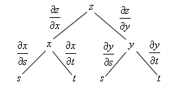
We start at the top with the function itself and the branch out from that point. The first set of branches is for the variables in the function. From each of these endpoints we put down a further set of branches that gives the variables that both \(x\) and \(y\) are a function of. We connect each letter with a line and each line represents a partial derivative as shown. Note that the letter in the numerator of the partial derivative is the upper “node” of the tree and the letter in the denominator of the partial derivative is the lower “node” of the tree.
To use this to get the chain rule we start at the bottom and for each branch that ends with the variable we want to take the derivative with respect to (\(s\) in this case) we move up the tree until we hit the top multiplying the derivatives that we see along that set of branches. Once we’ve done this for each branch that ends at \(s\), we then add the results up to get the chain rule for that given situation.
Note that we don’t always put the derivatives in the tree. Some of the trees get a little large/messy and so we won’t put in the derivatives. Just remember what derivative should be on each branch and you’ll be okay without actually writing them down.
Let’s write down some chain rules.
- \(\displaystyle \frac{{dw}}{{dt}}\) for \(w = f\left( {x,y,z} \right)\), \(x = {g_1}\left( t \right)\), \(y = {g_2}\left( t \right)\), and \(z = {g_3}\left( t \right)\)
- \(\displaystyle \frac{{\partial w}}{{\partial r}}\) for \(w = f\left( {x,y,z} \right)\), \(x = {g_1}\left( {s,t,r} \right)\), \(y = {g_2}\left( {s,t,r} \right)\), and \(z = {g_3}\left( {s,t,r} \right)\)
So, we’ll first need the tree diagram so let’s get that.
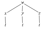
From this it looks like the chain rule for this case should be,
\[\frac{{dw}}{{dt}} = \frac{{\partial f}}{{\partial x}}\frac{{dx}}{{dt}} + \frac{{\partial f}}{{\partial y}}\frac{{dy}}{{dt}} + \frac{{\partial f}}{{\partial z}}\frac{{dz}}{{dt}}\]which is really just a natural extension to the two variable case that we saw above.
b \(\displaystyle \frac{{\partial w}}{{\partial r}}\) for \(w = f\left( {x,y,z} \right)\), \(x = {g_1}\left( {s,t,r} \right)\), \(y = {g_2}\left( {s,t,r} \right)\), and \(z = {g_3}\left( {s,t,r} \right)\) Show Solution
Here is the tree diagram for this situation.
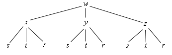
From this it looks like the derivative will be,
\[\frac{{\partial w}}{{\partial r}} = \frac{{\partial f}}{{\partial x}}\frac{{\partial x}}{{\partial r}} + \frac{{\partial f}}{{\partial y}}\frac{{\partial y}}{{\partial r}} + \frac{{\partial f}}{{\partial z}}\frac{{\partial z}}{{\partial r}}\]So, provided we can write down the tree diagram, and these aren’t usually too bad to write down, we can do the chain rule for any set up that we might run across.
We’ve now seen how to take first derivatives of these more complicated situations, but what about higher order derivatives? How do we do those? It’s probably easiest to see how to deal with these with an example.
We will need the first derivative before we can even think about finding the second derivative so let’s get that. This situation falls into the second case that we looked at above so we don’t need a new tree diagram. Here is the first derivative.
\[\begin{align*}\frac{{\partial f}}{{\partial \theta }} & = \frac{{\partial f}}{{\partial x}}\frac{{\partial x}}{{\partial \theta }} + \frac{{\partial f}}{{\partial y}}\frac{{\partial y}}{{\partial \theta }}\\ & = - r\sin \left( \theta \right)\frac{{\partial f}}{{\partial x}} + r\cos \left( \theta \right)\frac{{\partial f}}{{\partial y}}\end{align*}\]Okay, now we know that the second derivative is,
\[\frac{{{\partial ^2}f}}{{\partial {\theta ^2}}} = \frac{\partial }{{\partial \theta }}\left( {\frac{{\partial f}}{{\partial \theta }}} \right) = \frac{\partial }{{\partial \theta }}\left( { - r\sin \left( \theta \right)\frac{{\partial f}}{{\partial x}} + r\cos \left( \theta \right)\frac{{\partial f}}{{\partial y}}} \right)\]The issue here is to correctly deal with this derivative. Since the two first order derivatives, \(\frac{{\partial f}}{{\partial x}}\) and \(\frac{{\partial f}}{{\partial y}}\), are both functions of \(x\) and \(y\) which are in turn functions of \(r\) and \(\theta \) both of these terms are products. So, the using the product rule gives the following,
\[\frac{{{\partial ^2}f}}{{\partial {\theta ^2}}} = - r\cos \left( \theta \right)\frac{{\partial f}}{{\partial x}} - r\sin \left( \theta \right)\frac{\partial }{{\partial \theta }}\left( {\frac{{\partial f}}{{\partial x}}} \right) - r\sin \left( \theta \right)\frac{{\partial f}}{{\partial y}} + r\cos \left( \theta \right)\frac{\partial }{{\partial \theta }}\left( {\frac{{\partial f}}{{\partial y}}} \right)\]We now need to determine what \(\frac{\partial }{{\partial \theta }}\left( {\frac{{\partial f}}{{\partial x}}} \right)\) and \(\frac{\partial }{{\partial \theta }}\left( {\frac{{\partial f}}{{\partial y}}} \right)\) will be. These are both chain rule problems again since both of the derivatives are functions of \(x\) and \(y\) and we want to take the derivative with respect to \(\theta \).
Before we do these let’s rewrite the first chain rule that we did above a little.
\[\begin{equation}\frac{\partial }{{\partial \theta }}\left( f \right) = - r\sin \left( \theta \right)\frac{\partial }{{\partial x}}\left( f \right) + r\cos \left( \theta \right)\frac{\partial }{{\partial y}}\left( f \right) \label{eq:eq1} \end{equation}\]Note that all we’ve done is change the notation for the derivative a little. With the first chain rule written in this way we can think of \(\eqref{eq:eq1}\) as a formula for differentiating any function of \(x\) and \(y\) with respect to \(\theta \) provided we have \(x = r\cos \theta \) and \(y = r\sin \theta \).
This however is exactly what we need to do the two new derivatives we need above. Both of the first order partial derivatives, \(\frac{{\partial f}}{{\partial x}}\) and \(\frac{{\partial f}}{{\partial y}}\), are functions of \(x\) and \(y\) and \(x = r\cos \theta \) and \(y = r\sin \theta \) so we can use \(\eqref{eq:eq1}\) to compute these derivatives.
To do this we’ll simply replace all the f ’s in \(\eqref{eq:eq1}\) with the first order partial derivative that we want to differentiate. At that point all we need to do is a little notational work and we’ll get the formula that we’re after.
Here is the use of \(\eqref{eq:eq1}\) to compute \(\frac{\partial }{{\partial \theta }}\left( {\frac{{\partial f}}{{\partial x}}} \right)\).
\[\begin{align*}\frac{\partial }{{\partial \theta }}\left( {\frac{{\partial f}}{{\partial x}}} \right) & = - r\sin \left( \theta \right)\frac{\partial }{{\partial x}}\left( {\frac{{\partial f}}{{\partial x}}} \right) + r\cos \left( \theta \right)\frac{\partial }{{\partial y}}\left( {\frac{{\partial f}}{{\partial x}}} \right)\\ & = - r\sin \left( \theta \right)\frac{{{\partial ^2}f}}{{\partial {x^2}}} + r\cos \left( \theta \right)\frac{{{\partial ^2}f}}{{\partial y\partial x}}\end{align*}\]Here is the computation for \(\frac{\partial }{{\partial \theta }}\left( {\frac{{\partial f}}{{\partial y}}} \right)\).
\[\begin{align*}\frac{\partial }{{\partial \theta }}\left( {\frac{{\partial f}}{{\partial y}}} \right) & = - r\sin \left( \theta \right)\frac{\partial }{{\partial x}}\left( {\frac{{\partial f}}{{\partial y}}} \right) + r\cos \left( \theta \right)\frac{\partial }{{\partial y}}\left( {\frac{{\partial f}}{{\partial y}}} \right)\\ & = - r\sin \left( \theta \right)\frac{{{\partial ^2}f}}{{\partial x\partial y}} + r\cos \left( \theta \right)\frac{{{\partial ^2}f}}{{\partial {y^2}}}\end{align*}\]The final step is to plug these back into the second derivative and do some simplifying.
\[\begin{align*}\frac{{{\partial ^2}f}}{{\partial {\theta ^2}}} & = - r\cos \left( \theta \right)\frac{{\partial f}}{{\partial x}} - r\sin \left( \theta \right)\left( { - r\sin \left( \theta \right)\frac{{{\partial ^2}f}}{{\partial {x^2}}} + r\cos \left( \theta \right)\frac{{{\partial ^2}f}}{{\partial y\partial x}}} \right) - \\ & \hspace{0.25in}r\sin \left( \theta \right)\frac{{\partial f}}{{\partial y}} + r\cos \left( \theta \right)\left( { - r\sin \left( \theta \right)\frac{{{\partial ^2}f}}{{\partial x\partial y}} + r\cos \left( \theta \right)\frac{{{\partial ^2}f}}{{\partial {y^2}}}} \right)\\ & = - r\cos \left( \theta \right)\frac{{\partial f}}{{\partial x}} + {r^2}{\sin ^2}\left( \theta \right)\frac{{{\partial ^2}f}}{{\partial {x^2}}} - {r^2}\sin \left( \theta \right)\cos \left( \theta \right)\frac{{{\partial ^2}f}}{{\partial y\partial x}} - \\ & \hspace{0.25in}r\sin \left( \theta \right)\frac{{\partial f}}{{\partial y}} - {r^2}\sin \left( \theta \right)\cos \left( \theta \right)\frac{{{\partial ^2}f}}{{\partial x\partial y}} + {r^2}{\cos ^2}\left( \theta \right)\frac{{{\partial ^2}f}}{{\partial {y^2}}}\\ & = - r\cos \left( \theta \right)\frac{{\partial f}}{{\partial x}} - r\sin \left( \theta \right)\frac{{\partial f}}{{\partial y}} + {r^2}{\sin ^2}\left( \theta \right)\frac{{{\partial ^2}f}}{{\partial {x^2}}} - \\ & \hspace{0.5in}2{r^2}\sin \left( \theta \right)\cos \left( \theta \right)\frac{{{\partial ^2}f}}{{\partial y\partial x}} + {r^2}{\cos ^2}\left( \theta \right)\frac{{{\partial ^2}f}}{{\partial {y^2}}}\end{align*}\]It’s long and fairly messy but there it is.
The final topic in this section is a revisiting of implicit differentiation. With these forms of the chain rule implicit differentiation actually becomes a fairly simple process. Let’s start out with the implicit differentiation that we saw in a Calculus I course.
We will start with a function in the form \(F\left( {x,y} \right) = 0\) (if it’s not in this form simply move everything to one side of the equal sign to get it into this form) where \(y = y\left( x \right)\). In a Calculus I course we were then asked to compute \(\frac{{dy}}{{dx}}\) and this was often a fairly messy process. Using the chain rule from this section however we can get a nice simple formula for doing this. We’ll start by differentiating both sides with respect to \(x\). This will mean using the chain rule on the left side and the right side will, of course, differentiate to zero. Here are the results of that.
\[{F_x} + {F_y}\frac{{dy}}{{dx}} = 0\hspace{0.5in} \Rightarrow \hspace{0.5in}\frac{{dy}}{{dx}} = - \frac{{{F_x}}}{{{F_y}}}\]As shown, all we need to do next is solve for \(\frac{{dy}}{{dx}}\) and we’ve now got a very nice formula to use for implicit differentiation. Note as well that in order to simplify the formula we switched back to using the subscript notation for the derivatives.
Let’s check out a quick example.
The first step is to get a zero on one side of the equal sign and that’s easy enough to do.
\[x\cos \left( {3y} \right) + {x^3}{y^5} - 3x + {{\bf{e}}^{xy}} = 0\]Now, the function on the left is \(F\left( {x,y} \right)\) in our formula so all we need to do is use the formula to find the derivative.
\[\frac{{dy}}{{dx}} = - \frac{{\cos \left( {3y} \right) + 3{x^2}{y^5} - 3 + y{{\bf{e}}^{xy}}}}{{ - 3x\sin \left( {3y} \right) + 5{x^3}{y^4} + x{{\bf{e}}^{xy}}}}\]There we go. It would have taken much longer to do this using the old Calculus I way of doing this.
We can also do something similar to handle the types of implicit differentiation problems involving partial derivatives like those we saw when we first introduced partial derivatives. In these cases we will start off with a function in the form \(F\left( {x,y,z} \right) = 0\) and assume that \(z = f\left( {x,y} \right)\) and we want to find \(\frac{{\partial z}}{{\partial x}}\) and/or \(\frac{{\partial z}}{{\partial y}}\).
Let’s start by trying to find \(\frac{{\partial z}}{{\partial x}}\). We will differentiate both sides with respect to \(x\) and we’ll need to remember that we’re going to be treating \(y\) as a constant. Also, the left side will require the chain rule. Here is this derivative.
\[\frac{{\partial F}}{{\partial x}}\frac{{\partial x}}{{\partial x}} + \frac{{\partial F}}{{\partial y}}\frac{{\partial y}}{{\partial x}} + \frac{{\partial F}}{{\partial z}}\frac{{\partial z}}{{\partial x}} = 0\]Now, we have the following,
\[\frac{{\partial x}}{{\partial x}} = 1\hspace{0.5in}{\mbox{and }}\hspace{0.5in}\frac{{\partial y}}{{\partial x}} = 0\]The first is because we are just differentiating \(x\) with respect to \(x\) and we know that is 1. The second is because we are treating the \(y\) as a constant and so it will differentiate to zero.
Plugging these in and solving for \(\frac{{\partial z}}{{\partial x}}\) gives,
\[\frac{{\partial z}}{{\partial x}} = - \frac{{{F_x}}}{{{F_z}}}\]A similar argument can be used to show that,
\[\frac{{\partial z}}{{\partial y}} = - \frac{{{F_y}}}{{{F_z}}}\]As with the one variable case we switched to the subscripting notation for derivatives to simplify the formulas. Let’s take a quick look at an example of this.
This was one of the functions that we used the old implicit differentiation on back in the Partial Derivatives section. You might want to go back and see the difference between the two.
First let’s get everything on one side.
\[{x^2}\sin \left( {2y - 5z} \right) - 1 - y\cos \left( {6zx} \right) = 0\]Now, the function on the left is \(F\left( {x,y,z} \right)\) and so all that we need to do is use the formulas developed above to find the derivatives.
\[\frac{{\partial z}}{{\partial x}} = - \frac{{2x\sin \left( {2y - 5z} \right) + 6yz\sin \left( {6zx} \right)}}{{ - 5{x^2}\cos \left( {2y - 5z} \right) + 6yx\sin \left( {6zx} \right)}}\] \[\frac{{\partial z}}{{\partial y}} = - \frac{{2{x^2}\cos \left( {2y - 5z} \right) - \cos \left( {6zx} \right)}}{{ - 5{x^2}\cos \left( {2y - 5z} \right) + 6yx\sin \left( {6zx} \right)}}\]If you go back and compare these answers to those that we found the first time around you will notice that they might appear to be different. However, if you take into account the minus sign that sits in the front of our answers here you will see that they are in fact the same.