Section 16.1 : Vector Fields
We need to start this chapter off with the definition of a vector field as they will be a major component of both this chapter and the next. Let’s start off with the formal definition of a vector field.
Definition
A vector field on two (or three) dimensional space is a function \(\vec F\) that assigns to each point \(\left( {x,y} \right)\) (or \(\left( {x,y,z} \right)\)) a two (or three dimensional) vector given by \(\vec F\left( {x,y} \right)\) (or \(\vec F\left( {x,y,z} \right)\)).
That may not make a lot of sense, but most people do know what a vector field is, or at least they’ve seen a sketch of a vector field. If you’ve seen a current sketch giving the direction and magnitude of a flow of a fluid or the direction and magnitude of the winds then you’ve seen a sketch of a vector field.
The standard notation for the function \(\vec F\) is,
\[\begin{align*}\vec F\left( {x,y} \right) & = P\left( {x,y} \right)\vec i + Q\left( {x,y} \right)\vec j\\ \vec F\left( {x,y,z} \right) & = P\left( {x,y,z} \right)\vec i + Q\left( {x,y,z} \right)\vec j + R\left( {x,y,z} \right)\vec k\end{align*}\]depending on whether or not we’re in two or three dimensions. The function \(P\), \(Q\), \(R\) (if it is present) are sometimes called scalar functions.
Let’s take a quick look at a couple of examples.
- \(\vec F\left( {x,y} \right) = - y\,\vec i + x\,\vec j\)
- \(\vec F\left( {x,y,z} \right) = 2x\,\vec i - 2y\,\vec j - 2x\,\vec k\)
Okay, to graph the vector field we need to get some “values” of the function. This means plugging in some points into the function. Here are a couple of evaluations.
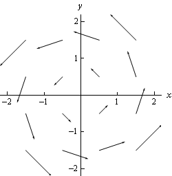
\[\begin{align*}\vec F\left( {\frac{1}{2},\frac{1}{2}} \right) & = - \frac{1}{2}\vec i + \frac{1}{2}\vec j\\ \vec F\left( {\frac{1}{2}, - \frac{1}{2}} \right) & = - \left( { - \frac{1}{2}} \right)\vec i + \frac{1}{2}\vec j = \frac{1}{2}\vec i + \frac{1}{2}\vec j\\\vec F\left( {\frac{3}{2},\frac{1}{4}} \right) & = - \frac{1}{4}\vec i + \frac{3}{2}\vec j\end{align*}\]So, just what do these evaluations tell us? Well the first one tells us that at the point \(\left( {\frac{1}{2},\frac{1}{2}} \right)\) we will plot the vector \( - \frac{1}{2}\vec i + \frac{1}{2}\vec j\). Likewise, the third evaluation tells us that at the point \(\left( {\frac{3}{2},\frac{1}{4}} \right)\) we will plot the vector \( - \frac{1}{4}\vec i + \frac{3}{2}\vec j\).
We can continue in this fashion plotting vectors for several points and we’ll get the following sketch of the vector field.
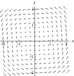
If we want significantly more points plotted, then it is usually best to use a computer aided graphing system such as Maple or Mathematica. Here is a sketch with many more vectors included that was generated with Mathematica.
b \(\vec F\left( {x,y,z} \right) = 2x\,\vec i - 2y\,\vec j - 2x\,\vec k\) Show Solution
In the case of three dimensional vector fields it is almost always better to use Maple, Mathematica, or some other such tool. Despite that let’s go ahead and do a couple of evaluations anyway.
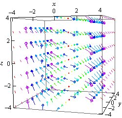
\[\begin{align*}\vec F\left( {1, - 3,2} \right) & = 2\,\vec i + 6\,\vec j - 2\,\vec k\\ \vec F\left( {0,5,3} \right) & = - 10\,\vec j\end{align*}\]Notice that \(z\) only affects the placement of the vector in this case and does not affect the direction or the magnitude of the vector. Sometimes this will happen so don’t get excited about it when it does.
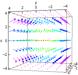
Here is a couple of sketches generated by Mathematica. The sketch on the left is from the “front” and the sketch on the right is from “above”.
Now that we’ve seen a couple of vector fields let’s notice that we’ve already seen a vector field function. In the second chapter we looked at the gradient vector. Recall that given a function \(f\left( {x,y,z} \right)\) the gradient vector is defined by,
This is a vector field and is often called a gradient vector field.
In these cases, the function \(f\left( {x,y,z} \right)\) is often called a scalar function to differentiate it from the vector field.
- \(f\left( {x,y} \right) = {x^2}\sin \left( {5y} \right)\)
- \(f\left( {x,y,z} \right) = z{{\bf{e}}^{ - xy}}\)
Note that we only gave the gradient vector definition for a three dimensional function, but don’t forget that there is also a two dimension definition. All that we need to drop off the third component of the vector.
Here is the gradient vector field for this function.
\[\nabla f = \left\langle {2x\sin \left( {5y} \right),5{x^2}\cos \left( {5y} \right)} \right\rangle \]b \(f\left( {x,y,z} \right) = z{{\bf{e}}^{ - xy}}\) Show Solution
There isn’t much to do here other than take the gradient.
\[\nabla f = \left\langle { - yz{{\bf{e}}^{ - xy}}, - xz{{\bf{e}}^{ - xy}},{{\bf{e}}^{ - xy}}} \right\rangle \]Let’s do another example that will illustrate the relationship between the gradient vector field of a function and its contours.
Recall that the contours for a function are nothing more than curves defined by,
\[f\left( {x,y} \right) = k\]for various values of \(k\). So, for our function the contours are defined by the equation,
\[{x^2} + {y^2} = k\]and so they are circles centered at the origin with radius \(\sqrt k \).
Here is the gradient vector field for this function.
\[\nabla f\left( {x,y} \right) = 2x\,\vec i + 2y\,\vec j\]Here is a sketch of several of the contours as well as the gradient vector field.
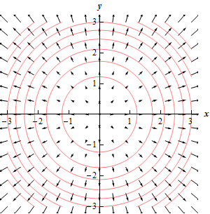
Notice that the vectors of the vector field are all orthogonal (or perpendicular) to the contours. This will always be the case when we are dealing with the contours of a function as well as its gradient vector field.
The \(k\)’s we used for the graph above were 1.5, 3, 4.5, 6, 7.5, 9, 10.5, 12, and 13.5. Now notice that as we increased \(k\) by 1.5 the contour curves get closer together and that as the contour curves get closer together the larger the vectors become. In other words, the closer the contour curves are (as \(k\) is increased by a fixed amount) the faster the function is changing at that point. Also recall that the direction of fastest change for a function is given by the gradient vector at that point. Therefore, it should make sense that the two ideas should match up as they do here.
The final topic of this section is that of conservative vector fields. A vector field \(\vec F\) is called a conservative vector field if there exists a function \(f\) such that \(\vec F = \nabla f\). If \(\vec F\) is a conservative vector field then the function, \(f\), is called a potential function for \(\vec F\).
All this definition is saying is that a vector field is conservative if it is also a gradient vector field for some function.
For instance the vector field \(\vec F = y\,\vec i + x\,\vec j\) is a conservative vector field with a potential function of \(f\left( {x,y} \right) = xy\) because \(\nabla f = \left\langle {y,x} \right\rangle \).
On the other hand, \(\vec F = - y\,\vec i + x\,\vec j\) is not a conservative vector field since there is no function \(f\) such that \(\vec F = \nabla f\). If you’re not sure that you believe this at this point be patient, we will be able to prove this in a couple of sections. In that section we will also show how to find the potential function for a conservative vector field.