Algebra - Graphing Polynomials

Show Mobile Notice Show All Notes Hide All Notes

Mobile Notice

You appear to be on a device with a "narrow" screen width (i.e. you are probably on a mobile phone). Due to the nature of the mathematics on this site it is best views in landscape mode. If your device is not in landscape mode many of the equations will run off the side of your device (should be able to scroll to see them) and some of the menu items will be cut off due to the narrow screen width.

Section 5.3 : Graphing Polynomials

In this section we are going to look at a method for getting a rough sketch of a general polynomial. The only real information that we’re going to need is a complete list of all the zeroes (including multiplicity) for the polynomial.

In this section we are going to either be given the list of zeroes or they will be easy to find. In the next section we will go into a method for determining a large portion of the list for most polynomials. We are graphing first since the method for finding all the zeroes of a polynomial can be a little long and we don’t want to obscure the details of this section in the mess of finding the zeroes of the polynomial.

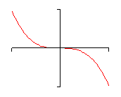
Let’s start off with the graph of couple of polynomials.

There are two graphs in this image. The domain of the graph on the left is from -5 to 5 while the range is from -400 to 400. The graph starts at approximately (-5,400) in the 2nd quadrant and decreases into the 3rd quadrant to a valley at approximately (-3,-180). It then increases and passes through the origin into the 1st quadrant horizontally. The graph increases from this point to a peak at approximately (3,180) and then decreases into the 4th quadrant ending at approximately (5,-400). The domain of the graph on the right is from -5 to 5 while the range is from -30 to 100. The graph starts at approximately (-5,100) in the 2nd quadrant and decreases into the 3rd quadrant to a valley at approximately (-3,-20). It then increases back into the 2nd quadrant to a peak at (0, 30). It then passes into the 1st quadrant and decreases into the 4th quadrant to a valley at approximately (3,-20). It then increases back into the 1st quadrant ending at approximately (5,100).

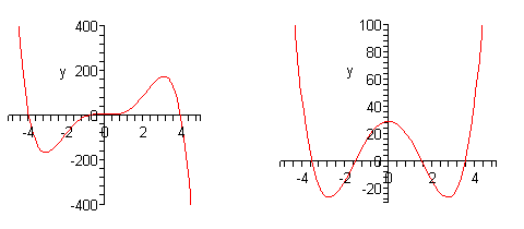
Do not worry about the equations for these polynomials. We are giving these only so we can use them to illustrate some ideas about polynomials.

First, notice that the graphs are nice and smooth. There are no holes or breaks in the graph and there are no sharp corners in the graph. The graphs of polynomials will always be nice smooth curves.

Secondly, the “humps” where the graph changes direction from increasing to decreasing or decreasing to increasing are often called turning points. If we know that the polynomial has degree $n$ then we will know that there will be at most $n - 1$ turning points in the graph.

While this won’t help much with the actual graphing process it will be a nice check. If we have a fourth degree polynomial with 5 turning point then we will know that we’ve done something wrong since a fourth degree polynomial will have no more than 3 turning points.

Next, we need to explore the relationship between the $x$-intercepts of a graph of a polynomial and the zeroes of the polynomial. Recall that to find the $x$-intercepts of a function we need to solve the equation

\[P\left( x \right) = 0\]

Also, recall that $x = r$ is a zero of the polynomial, $P\left( x \right)$, provided $P\left( r \right) = 0$. But this means that $x = r$ is also a solution to $P\left( x \right) = 0$.

In other words, the zeroes of a polynomial are also the x-intercepts of the graph. Also, recall that $x$-intercepts can either cross the $x$-axis or they can just touch the $x$-axis without actually crossing the axis.

Notice as well from the graphs above that the $x$-intercepts can either flatten out as they cross the $x$-axis or they can go through the $x$-axis at an angle.

The following fact will relate all of these ideas to the multiplicity of the zero.

Fact

If $x = r$ is a zero of the polynomial $P\left( x \right)$ with multiplicity $k$ then,

If $k$ is odd then the $x$-intercept corresponding to $x = r$ will cross the $x$-axis.
If $k$ is even then the $x$-intercept corresponding to $x = r$ will only touch the $x$-axis and not actually cross it.

Furthermore, if $k > 1$ then the graph will flatten out at $x = r$.

Finally, notice that as we let $x$ get large in both the positive or negative sense (i.e. at either end of the graph) then the graph will either increase without bound or decrease without bound. This will always happen with every polynomial and we can use the following test to determine just what will happen at the endpoints of the graph.

Leading Coefficient Test

Suppose that $P\left( x \right)$ is a polynomial with degree $n$. So we know that the polynomial must look like,

\[P\left( x \right) = a{x^n} + \cdots \]

We don’t know if there are any other terms in the polynomial, but we do know that the first term will have to be the one listed since it has degree $n$. We now have the following facts about the graph of $P\left( x \right)$ at the ends of the graph.

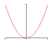
If $a > 0$ and $n$ is even then the graph of $P\left( x \right)$ will increase without bound at both endpoints. A good example of this is the graph of x².
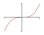
If $a > 0$ and $n$ is odd then the graph of $P\left( x \right)$ will increase without bound at the right end and decrease without bound at the left end. A good example of this is the graph of x³.
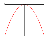
$There are no tick marks on the x or y-axis on this graph. This is just a typical $x^{3}$ graph. It starts in the lower left corner of the 3rd quadrant and increases until it passes through the origin horizontally and then increases up into the upper right corner of the 1st quadrant.$
If $a < 0$ and $n$ is even then the graph of $P\left( x \right)$ will decrease without bound at both endpoints. A good example of this is the graph of -x².
If $a < 0$ and $n$ is odd then the graph of $P\left( x \right)$ will decrease without bound at the right end and increase without bound at the left end. A good example of this is the graph of -x³.
$There are no tick marks on the x or y-axis on this graph. This is just a typical $x^{3}$ graph except it have been flipped around the x-axis. It starts in the upper left corner of the 2nd quadrant and decreases until it passes through the origin horizontally and then decreases down into the lower right corner of the 4th quadrant.$

Okay, now that we’ve got all that out of the way we can finally give a process for getting a rough sketch of the graph of a polynomial.

Process for Graphing a Polynomial

Determine all the zeroes of the polynomial and their multiplicity. Use the fact above to determine the $x$-intercept that corresponds to each zero will cross the $x$-axis or just touch it and if the $x$-intercept will flatten out or not.
Determine the $y$-intercept, $\left( {0,P\left( 0 \right)} \right)$.
Use the leading coefficient test to determine the behavior of the polynomial at the end of the graph.
Plot a few more points. This is left intentionally vague. The more points that you plot the better the sketch. At the least you should plot at least one at either end of the graph and at least one point between each pair of zeroes.

We should give a quick warning about this process before we actually try to use it. This process assumes that all the zeroes are real numbers. If there are any complex zeroes then this process may miss some pretty important features of the graph.

Let’s sketch a couple of polynomials.

Example 1 Sketch the graph of $P\left( x \right) = 5{x^5} - 20{x^4} + 5{x^3} + 50{x^2} - 20x - 40$.

Show Solution

We found the zeroes and multiplicities of this polynomial in the previous section so we’ll just write them back down here for reference purposes.

\[\begin{align*}x & = - 1 & \hspace{0.25in} & \left( {{\mbox{multiplicity 2}}} \right)\\ x & = 2 & \hspace{0.25in}&\left( {{\mbox{multiplicity 3}}} \right)\end{align*}\]

So, from the fact we know that $x = - 1$ will just touch the $x$-axis and not actually cross it and that $x = 2$ will cross the $x$-axis and will be flat as it does this since the multiplicity is greater than 1. Also, both will be flat as they cross the $x$-axis since the multiplicity for both is greater than 1.

Next, the $y$-intercept is $\left( {0, - 40} \right)$.

The coefficient of the 5^th degree term is positive and since the degree is odd we know that this polynomial will increase without bound at the right end and decrease without bound at the left end.

Finally, we just need to evaluate the polynomial at a couple of points. The points that we pick aren’t really all that important. We just want to pick points according to the guidelines in the process outlined above and points that will be fairly easy to evaluate. Here are some points. We will leave it to you to verify the evaluations.

\[P\left( { - 2} \right) = - 320\hspace{0.25in}\hspace{0.25in}P\left( 1 \right) = - 20\hspace{0.25in}\hspace{0.25in}P\left( 3 \right) = 80\]

Now, to actually sketch the graph we’ll start on the left end and work our way across to the right end. First, we know that on the left end the graph decreases without bound as we make $x$ more and more negative and this agrees with the point that we evaluated at $x = - 2$.

So, as we move to the right the function will actually be increasing at $x = - 2$ and we will continue to increase until we hit the first x-intercept at $x = - 1$. At this point we know that the graph just touches the $x$-axis without actually crossing it and will be flat as it does this. This means that at $x = -1$ the graph must be a turning point.

The graph is now decreasing as we move to the right. Again, this agrees with the next point that we’ll run across, the $y$-intercept.

Now, according to the next point that we’ve got, $x = 1$, the graph must have another turning point somewhere between $x = 0$ and $x = 1$ since the graph is higher at $x = 1$ than at $x = 0$. Just where this turning point will occur is very difficult to determine at this level so we won’t worry about trying to find it. In fact, determining this point usually requires some Calculus.

So, we are moving to the right and the function is increasing. The next point that we hit is the $x$-intercept at $x = 2$ and this one crosses the $x$-axis so we know that there won’t be a turning point here as there was at the first $x$-intercept. Also, the graph will be flat as it touches the $x$-axis because the multiplicity is greater than one. So, the graph will continue to increase through this point, briefly flattening out as it touches the $x$-axis, until we hit the final point that we evaluated the function at $x = 3$.

At this point we’ve hit all the $x$-intercepts and we know that the graph will increase without bound at the right end and so it looks like all we need to do is sketch in an increasing curve.

Here is a sketch of the polynomial.

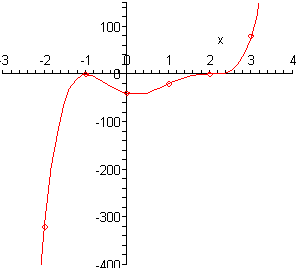
The domain of this graph is from -3 to 4 while the range is from -400 to 150. The graph starts in the 3rd quadrant at (-2,-320) and increases to a peak at (-1,0). It then decreases to a valley at (0,-40) and increases up through the point (1,-20) and crosses the x-axis horizontally at (2,0) and then continues to increase ending at (3,80).

Note that one of the reasons for plotting points at the ends is to see just how fast the graph is increasing or decreasing. We can see from the evaluations that the graph is decreasing on the left end much faster than it’s increasing on the right end.

Okay, let’s take a look at another polynomial. This time we’ll go all the way through the process of finding the zeroes.

Example 2 Sketch the graph of $P\left( x \right) = {x^4} - {x^3} - 6{x^2}$.

Show Solution

First, we’ll need to factor this polynomial as much as possible so we can identify the zeroes and get their multiplicities.

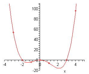
\[P\left( x \right) = {x^4} - {x^3} - 6{x^2} = {x^2}\left( {{x^2} - x - 6} \right) = {x^2}\left( {x - 3} \right)\left( {x + 2} \right)\]

Here is a list of the zeroes and their multiplicities.

\[\begin{align*}x & = - 2 & \hspace{0.25in} & \left( {{\mbox{multiplicity 1}}} \right)\\ x & = 0 & \hspace{0.25in} & \left( {{\mbox{multiplicity 2}}} \right)\\ x & = 3 & \hspace{0.25in} & \left( {{\mbox{multiplicity 1}}} \right)\end{align*}\]

So, the zeroes at $x = - 2$ and $x = 3$ will correspond to $x$-intercepts that cross the $x$-axis since their multiplicity is odd and will do so at an angle since their multiplicity is NOT at least 2. The zero at $x = 0$ will not cross the $x$-axis since its multiplicity is even but will be flat as it touches the $x$-axis since the multiplicity is greater than one.

The $y$-intercept is $\left( {0,0} \right)$ and notice that this is also an $x$-intercept.

The coefficient of the 4^th degree term is positive and so since the degree is even we know that the polynomial will increase without bound at both ends of the graph.

Finally, here are some function evaluations.

\[P\left( { - 3} \right) = 54\hspace{0.25in}P\left( { - 1} \right) = - 4\hspace{0.25in}P\left( 1 \right) = - 6\hspace{0.25in}P\left( 4 \right) = 96\]

Now, starting at the left end we know that as we make $x$ more and more negative the function must increase without bound. That means that as we move to the right the graph will actually be decreasing.

At $x = - 3$ the graph will be decreasing and will continue to decrease when we hit the first $x$-intercept at $x = - 2$ since we know that this $x$-intercept will cross the $x$-axis.

Next, since the next $x$-intercept is at $x = 0$ we will have to have a turning point somewhere so that the graph can increase back up to this $x$-intercept. Again, we won’t worry about where this turning point actually is.

Once we hit the $x$-intercept at $x = 0$ we know that we’ve got to have a turning point since this $x$-intercept doesn’t cross the $x$-axis. Therefore, to the right of $x = 0$ the graph will now be decreasing. Recall however, that because the multiplicity is greater than one it will be flat as it touches the $x$-axis.

It will continue to decrease until it hits another turning point (at some unknown point) so that the graph can get back up to the $x$-axis for the next $x$-intercept at $x = 3$. This is the final $x$-intercept and since the graph is increasing at this point and must increase without bound at this end we are done.

Here is a sketch of the graph.

The domain of this graph is from -4 to 5 while the range is from -20 to 110. The graph starts in the 2nd quadrant at (-3,54) and decreases passing through the x-axis at (-2,0) into the 3rd quadrant and hits a valley at approximately (-1.5, -5). It then increases to a peak at the origin and then decreases into the 4th quadrant passing through the point (1,-6) and hitting a valley at approximately (2,-18). Finally it increases passing through the x-axis at (3,0) into the 1st quadrant ending at (4,96).

Example 3 Sketch the graph of $P\left( x \right) = - {x^5} + 4{x^3}$.

Show Solution

As with the previous example we’ll first need to factor this as much as possible.

\[P\left( x \right) = - {x^5} + 4{x^3} = - \left( {{x^5} - 4{x^3}} \right) = - {x^3}\left( {{x^2} - 4} \right) = - {x^3}\left( {x - 2} \right)\left( {x + 2} \right)\]

Notice that we first factored out a minus sign to make the rest of the factoring a little easier. Here is a list of all the zeroes and their multiplicities.

\[\begin{align*}x & = - 2 & \hspace{0.25in} & \left( {{\mbox{multiplicity 1}}} \right)\\ x & = 0 & \hspace{0.25in} & \left( {{\mbox{multiplicity 3}}} \right)\\ x & = 2 & \hspace{0.25in} & \left( {{\mbox{multiplicity 1}}} \right)\end{align*}\]

So, all three zeroes correspond to $x$-intercepts that actually cross the $x$-axis since all their multiplicities are odd, however, only the $x$-intercept at $x = 0$ will cross the $x$-axis flattened out.

The $y$-intercept is $\left( {0,0} \right)$ and as with the previous example this is also an $x$-intercept.

In this case the coefficient of the 5^th degree term is negative and so since the degree is odd the graph will increase without bound on the left side and decrease without bound on the right side.

Here are some function evaluations.

\[P\left( { - 3} \right) = 135\hspace{0.25in}\,\,\,P\left( { - 1} \right) = - 3\hspace{0.25in}\,\,\,\,\,P\left( 1 \right) = 3\hspace{0.25in}P\left( 3 \right) = - 135\]

Alright, this graph will start out much as the previous graph did. At the left end the graph will be decreasing as we move to the right and will decrease through the first $x$-intercept at $x = - 2$ since know that this $x$-intercept crosses the $x$-axis.

Now at some point we’ll get a turning point so the graph can get back up to the next $x$-intercept at $x = 0$ and the graph will continue to increase through this point since it also crosses the $x$-axis. Note as well that the graph should be flat at this point as well since the multiplicity is greater than one.

Finally, the graph will reach another turning point and start decreasing so it can get back down to the final $x$-intercept at $x = 2$. Since we know that the graph will decrease without bound at this end we are done.

Here is the sketch of this polynomial.

The domain of this graph is from -4 to 4 while the range is from -20 to 20. The graph starts in the 2nd quadrant at approximately (-2.5,20) and decreases passing through the x-axis at (-2,0) into the 3rd quadrant and hits a valley at approximately (-1.5, -6). It then increases up through the point (-1,-3) and then passing through the origin horizontally into the 1st quadrant. It goes though the point (1,3) reaches a peak at approximately (1.5,6). It then decreases passing through the x-axis at (2,0) into 4th quadrant ending at approximately (2.5,-20).

The process that we’ve used in these examples can be a difficult process to learn. It takes time to learn how to correctly interpret the results.

Also, as pointed out at various spots there are several situations that we won’t be able to deal with here. To find the majority of the turning points we would need some Calculus, which we clearly don’t have. Also, the process does require that we have all the zeroes and that they all be real numbers.

Even with these drawbacks however, the process can at least give us an idea of what the graph of a polynomial will look like.