Section 4.1 : The Definition
You know, it’s always a little scary when we devote a whole section just to the definition of something. Laplace transforms (or just transforms) can seem scary when we first start looking at them. However, as we will see, they aren’t as bad as they may appear at first.
Before we start with the definition of the Laplace transform we need to get another definition out of the way.
A function is called piecewise continuous on an interval if the interval can be broken into a finite number of subintervals on which the function is continuous on each open subinterval (i.e. the subinterval without its endpoints) and has a finite limit at the endpoints of each subinterval. Below is a sketch of a piecewise continuous function.
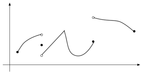
In other words, a piecewise continuous function is a function that has a finite number of breaks in it and doesn’t blow up to infinity anywhere.
Now, let’s take a look at the definition of the Laplace transform.
Definition
Suppose that \(f(t)\) is a piecewise continuous function. The Laplace transform of \(f(t)\) is denoted \(\mathcal{L}\left\{ {f\left( t \right)} \right\}\) and defined as
\[\begin{equation}\mathcal{L}\left\{ {f\left( t \right)} \right\} = \int_{{\,0}}^{{\,\infty }}{{{{\bf{e}}^{ - s\,t}}f\left( t \right)\,dt}}\label{eq:eq1}\end{equation}\]There is an alternate notation for Laplace transforms. For the sake of convenience we will often denote Laplace transforms as,
\[\mathcal{L}\left\{ {f\left( t \right)} \right\} = F\left( s \right)\]With this alternate notation, note that the transform is really a function of a new variable, \(s\), and that all the \(t\)’s will drop out in the integration process.
Now, the integral in the definition of the transform is called an improper integral and it would probably be best to recall how these kinds of integrals work before we actually jump into computing some transforms.
Remember that you need to convert improper integrals to limits as follows,
\[\int_{{\,0}}^{{\,\infty }}{{{{\bf{e}}^{c\,t}}\,dt}} = \mathop {\lim }\limits_{n \to \infty } \int_{{\,0}}^{{\,n}}{{{{\bf{e}}^{c\,t}}\,dt}}\]Now, do the integral, then evaluate the limit.
\[\begin{align*}\int_{{\,0}}^{{\,\infty }}{{{{\bf{e}}^{c\,t}}\,dt}} & = \mathop {\lim }\limits_{n \to \infty } \int_{{\,0}}^{{\,n}}{{{{\bf{e}}^{c\,t}}\,dt}}\\ & = \mathop {\lim }\limits_{n \to \infty } \left. {\left( {\frac{1}{c}{{\bf{e}}^{c\,t}}} \right)} \right|_0^n\\ & = \mathop {\lim }\limits_{n \to \infty } \left( {\frac{1}{c}{{\bf{e}}^{c\,n}} - \frac{1}{c}} \right)\end{align*}\]Now, at this point, we’ve got to be careful. The value of \(c\) will affect our answer. We’ve already assumed that \(c\) was non-zero, now we need to worry about the sign of \(c\). If \(c\) is positive the exponential will go to infinity. On the other hand, if \(c\) is negative the exponential will go to zero.
So, the integral is only convergent (i.e. the limit exists and is finite) provided \(c<0\). In this case we get,
\[\begin{equation}\int_{{\,0}}^{{\,\infty }}{{{{\bf{e}}^{c\,t}}\,dt}} = - \frac{1}{c}\hspace{0.25in}\hspace{0.25in}{\mbox{provided }}\,c < 0\label{eq:eq2}\end{equation}\]Now that we remember how to do these, let’s compute some Laplace transforms. We’ll start off with probably the simplest Laplace transform to compute.
There’s not really a whole lot do here other than plug the function \(f(t) = 1\) into \(\eqref{eq:eq1}\)
\[\mathcal{L}\left\{ 1 \right\} = \int_{{\,0}}^{{\,\infty }}{{{{\bf{e}}^{ - st}}\,dt}}\]Now, at this point notice that this is nothing more than the integral in the previous example with \(c = - s\). Therefore, all we need to do is reuse \(\eqref{eq:eq2}\) with the appropriate substitution. Doing this gives,
\[\mathcal{L}\left\{ 1 \right\} = \int_{{\,0}}^{{\,\infty }}{{{{\bf{e}}^{ - \,s\,t}}\,dt}} = - \frac{1}{{ - s}}\hspace{0.25in}\hspace{0.25in}{\mbox{provided }} - s < 0\]Or, with some simplification we have,
\[\mathcal{L}\left\{ 1 \right\} = \frac{1}{s}\hspace{0.25in}{\mbox{provided }}s > 0\]Notice that we had to put a restriction on \(s\) in order to actually compute the transform. All Laplace transforms will have restrictions on \(s\). At this stage of the game, this restriction is something that we tend to ignore, but we really shouldn’t ever forget that it’s there.
Let’s do another example.
Plug the function into the definition of the transform and do a little simplification.
\[\mathcal{L}\left\{ {{{\bf{e}}^{a\,t}}} \right\} = \int_{{\,0}}^{{\,\infty }}{{{{\bf{e}}^{ - s\,t}}{{\bf{e}}^{a\,t}}\,dt}} = \int_{{\,0}}^{{\,\infty }}{{{{\bf{e}}^{\left( {a - s} \right)t}}\,dt}}\]Once again, notice that we can use \(\eqref{eq:eq2}\) provided \(c = a - s\). So, let’s do this.
\[\begin{align*}\mathcal{L}\left\{ {{{\bf{e}}^{a\,t}}} \right\} & = \int_{{\,0}}^{{\,\infty }}{{{{\bf{e}}^{\left( {a - s} \right)t}}\,dt}}\\ & = - \frac{1}{{a - s}}\hspace{0.25in}\hspace{0.25in}{\mbox{provided }}a - s < 0\\ & = \frac{1}{{s - a}}\hspace{0.25in}\hspace{0.25in}\hspace{0.25in}{\mbox{provided }}s > a\end{align*}\]Let’s do one more example that doesn’t come down to an application of \(\eqref{eq:eq2}\).
Note that we’re going to leave it to you to check most of the integration here. Plug the function into the definition. This time let’s also use the alternate notation.
\[\begin{align*}\mathcal{L}\left\{ {\sin \left( {at} \right)} \right\} & = F\left( s \right)\\ & = \int_{{\,0}}^{{\,\infty }}{{{{\bf{e}}^{ - st}}\sin \left( {at} \right)\,dt}}\\ & = \mathop {\lim }\limits_{n \to \infty } \int_{{\,0}}^{{\,n}}{{{{\bf{e}}^{ - st}}\sin \left( {at} \right)\,dt}}\end{align*}\]Now, if we integrate by parts we will arrive at,
\[F\left( s \right) = \mathop {\lim }\limits_{n \to \infty } \left( { - \left. {\left( {\frac{1}{a}{{\bf{e}}^{ - st}}\cos \left( {at} \right)} \right)} \right|_0^n - \frac{s}{a}\int_{{\,0}}^{{\,n}}{{{{\bf{e}}^{ - st}}\cos \left( {at} \right)\,dt}}} \right)\]Now, evaluate the first term to simplify it a little and integrate by parts again on the integral. Doing this arrives at,
\[F\left( s \right) = \mathop {\lim }\limits_{n \to \infty } \left( {\frac{1}{a}\left( {1 - {{\bf{e}}^{ - sn}}\cos \left( {an} \right)} \right) - \frac{s}{a}\left( {\left. {\left( {\frac{1}{a}{{\bf{e}}^{ - st}}\sin \left( {at} \right)} \right)} \right|_0^n + \frac{s}{a}\int_{{\,0}}^{{\,n}}{{{{\bf{e}}^{ - st}}\sin \left( {at} \right)\,dt}}} \right)} \right)\]Now, evaluate the second term, take the limit and simplify.
\[\begin{align*}F\left( s \right) & = \mathop {\lim }\limits_{n \to \infty } \left( {\frac{1}{a}\left( {1 - {{\bf{e}}^{ - sn}}\cos \left( {an} \right)} \right) - \frac{s}{a}\left( {\frac{1}{a}{{\bf{e}}^{ - sn}}\sin \left( {an} \right) + \frac{s}{a}\int_{{\,0}}^{{\,n}}{{{{\bf{e}}^{ - st}}\sin \left( {at} \right)\,dt}}} \right)} \right)\\ & = \frac{1}{a} - \frac{s}{a}\left( {\frac{s}{a}\int_{{\,0}}^{{\,\infty }}{{{{\bf{e}}^{ - st}}\sin \left( {at} \right)\,dt}}} \right)\\ & = \frac{1}{a} - \frac{{{s^2}}}{{{a^2}}}\int_{{\,0}}^{{\,\infty }}{{{{\bf{e}}^{ - st}}\sin \left( {at} \right)\,dt}}\end{align*}\]Now, notice that in the limits we had to assume that \(s>0\) in order to do the following two limits.
\[\begin{align*}\mathop {\lim }\limits_{n \to \infty } {{\bf{e}}^{ - sn}}\cos \left( {an} \right) & = 0\\ \mathop {\lim }\limits_{n \to \infty } {{\bf{e}}^{ - sn}}\sin \left( {an} \right) & = 0\end{align*}\]Without this assumption, we get a divergent integral again. Also, note that when we got back to the integral we just converted the upper limit back to infinity. The reason for this is that, if you think about it, this integral is nothing more than the integral that we started with. Therefore, we now get,
\[F\left( s \right) = \frac{1}{a} - \frac{{{s^2}}}{{{a^2}}}F\left( s \right)\]Now, simply solve for \(F(s)\) to get,
\[\mathcal{L}\left\{ {\sin \left( {at} \right)} \right\} = F\left( s \right) = \frac{a}{{{s^2} + {a^2}}}\hspace{0.25in}\hspace{0.25in}{\mbox{provided }}s > 0\]As this example shows, computing Laplace transforms is often messy.
Before moving on to the next section, we need to do a little side note. On occasion you will see the following as the definition of the Laplace transform.
\[\mathcal{L}\left\{ {f\left( t \right)} \right\} = \int_{{\, - \infty }}^{{\,\infty }}{{{{\bf{e}}^{ - st}}f\left( t \right)\,dt}}\]Note the change in the lower limit from zero to negative infinity. In these cases there is almost always the assumption that the function \(f(t)\) is in fact defined as follows,
\[f\left( t \right) = \left\{ {\begin{array}{*{20}{l}}{f\left( t \right)}&{{\mbox{if }}t \ge 0}\\0&{{\mbox{if }}t < 0}\end{array}} \right.\]In other words, it is assumed that the function is zero if t<0. In this case the first half of the integral will drop out since the function is zero and we will get back to the definition given in \(\eqref{eq:eq1}\). A Heaviside function is usually used to make the function zero for t<0. We will be looking at these in a later section.