Paul's Online Notes
Paul's Online Notes
Home / Differential Equations / Systems of DE's / Phase Plane
Show Mobile Notice Show All Notes Hide All Notes
Mobile Notice
You appear to be on a device with a "narrow" screen width (i.e. you are probably on a mobile phone). Due to the nature of the mathematics on this site it is best views in landscape mode. If your device is not in landscape mode many of the equations will run off the side of your device (should be able to scroll to see them) and some of the menu items will be cut off due to the narrow screen width.

Section 5.6 : Phase Plane

Before proceeding with actually solving systems of differential equations there’s one topic that we need to take a look at. This is a topic that’s not always taught in a differential equations class but in case you’re in a course where it is taught we should cover it so that you are prepared for it.

Let’s start with a general homogeneous system,

\[\begin{equation}\vec x' = A\vec x\label{eq:eq1}\end{equation}\]

Notice that

\[\vec x = \vec 0\]

is a solution to the system of differential equations. What we’d like to ask is, do the other solutions to the system approach this solution as \(t\) increases or do they move away from this solution? We did something similar to this when we classified equilibrium solutions in a previous section. In fact, what we’re doing here is simply an extension of this idea to systems of differential equations.

The solution \(\vec x = \vec 0\) is called an equilibrium solution for the system. As with the single differential equations case, equilibrium solutions are those solutions for which

\[A\vec x = \vec 0\]

We are going to assume that \(A\) is a nonsingular matrix and hence will have only one solution,

\[\vec x = \vec 0\]

and so we will have only one equilibrium solution.

Back in the single differential equation case recall that we started by choosing values of \(y\) and plugging these into the function \(f(y)\) to determine values of \(y'\). We then used these values to sketch tangents to the solution at that particular value of \(y\). From this we could sketch in some solutions and use this information to classify the equilibrium solutions.

We are going to do something similar here, but it will be slightly different as well. First, we are going to restrict ourselves down to the \(2 \times 2\) case. So, we’ll be looking at systems of the form,

\[\begin{array}{*{20}{c}}\begin{align*}{{x'}_1} & = a{x_1} + b{x_2}\\ {{x'}_2} & = c{x_1} + d{x_2}\end{align*}&{\hspace{0.25in} \Rightarrow \hspace{0.25in}\hspace{0.25in}\vec x' = \left( {\begin{array}{*{20}{c}}a&b\\c&d\end{array}} \right)\vec x}\end{array}\]

Solutions to this system will be of the form,

\[\vec x = \left( {\begin{array}{*{20}{c}}{{x_1}\left( t \right)}\\{{x_2}\left( t \right)}\end{array}} \right)\]

and our single equilibrium solution will be,

\[\vec x = \left( {\begin{array}{*{20}{c}}0\\0\end{array}} \right)\]

In the single differential equation case we were able to sketch the solution, \(y(t)\) in the y-t plane and see actual solutions. However, this would somewhat difficult in this case since our solutions are actually vectors. What we’re going to do here is think of the solutions to the system as points in the \({x_1}\,{x_2}\) plane and plot these points. Our equilibrium solution will correspond to the origin of \({x_1}\,{x_2}\). plane and the \({x_1}\,{x_2}\) plane is called the phase plane.

To sketch a solution in the phase plane we can pick values of \(t\) and plug these into the solution. This gives us a point in the \({x_1}\,{x_2}\) or phase plane that we can plot. Doing this for many values of \(t\) will then give us a sketch of what the solution will be doing in the phase plane. A sketch of a particular solution in the phase plane is called the trajectory of the solution. Once we have the trajectory of a solution sketched we can then ask whether or not the solution will approach the equilibrium solution as \(t\) increases.

We would like to be able to sketch trajectories without actually having solutions in hand. There are a couple of ways to do this. We’ll look at one of those here and we’ll look at the other in the next couple of sections.

One way to get a sketch of trajectories is to do something similar to what we did the first time we looked at equilibrium solutions. We can choose values of \(\vec x\) (note that these will be points in the phase plane) and compute \(A\vec x\). This will give a vector that represents \(\vec x'\)at that particular solution. As with the single differential equation case this vector will be tangent to the trajectory at that point. We can sketch a bunch of the tangent vectors and then sketch in the trajectories.

This is a fairly work intensive way of doing these and isn’t the way to do them in general. However, it is a way to get trajectories without doing any solution work. All we need is the system of differential equations. Let’s take a quick look at an example.

Example 1 Sketch some trajectories for the system, \[\begin{array}{*{20}{c}}\begin{align*}{{x'}_1} & = {x_1} + 2{x_2}\\ {{x'}_2} & = 3{x_1} + 2{x_2}\end{align*}&{\hspace{0.25in} \Rightarrow \hspace{0.25in}\vec x' = \left( {\begin{array}{*{20}{c}}1&2\\3&2\end{array}} \right)\vec x}\end{array}\]
Show Solution

So, what we need to do is pick some points in the phase plane, plug them into the right side of the system. We’ll do this for a couple of points.

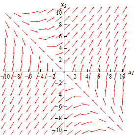
\[\begin{align*}\vec x & = \left( {\begin{array}{*{20}{c}}{ - 1}\\1\end{array}} \right) & \Rightarrow \hspace{0.25in}\vec x'& = \left( {\begin{array}{*{20}{c}}1&2\\3&2\end{array}} \right)\left( {\begin{array}{*{20}{c}}{ - 1}\\1\end{array}} \right) = \left( {\begin{array}{*{20}{c}}1\\{ - 1}\end{array}} \right)\\ \vec x & = \left( {\begin{array}{*{20}{c}}2\\0\end{array}} \right) & \Rightarrow \hspace{0.25in}\vec x' & = \left( {\begin{array}{*{20}{c}}1&2\\3&2\end{array}} \right)\left( {\begin{array}{*{20}{c}}2\\0\end{array}} \right) = \left( {\begin{array}{*{20}{c}}2\\6\end{array}} \right)\hspace{0.25in}\\ \vec x & = \left( {\begin{array}{*{20}{c}}{ - 3}\\{ - 2}\end{array}} \right) & \Rightarrow \hspace{0.25in}\vec x' & = \left( {\begin{array}{*{20}{c}}1&2\\3&2\end{array}} \right)\left( {\begin{array}{*{20}{c}}{ - 3}\\{ - 2}\end{array}} \right) = \left( {\begin{array}{*{20}{c}}{ - 7}\\{ - 13}\end{array}} \right)\hspace{0.25in}\end{align*}\]

So, what does this tell us? Well at the point \(\left( { - 1,1} \right)\) in the phase plane there will be a vector pointing in the direction \(\left\langle {1, - 1} \right\rangle \). At the point \(\left( {2,0} \right)\) there will be a vector pointing in the direction \(\left\langle {2,6} \right\rangle \). At the point \(\left( { - 3, - 2} \right)\) there will be a vector pointing in the direction \(\left\langle { - 7, - 13} \right\rangle \).

Doing this for a large number of points in the phase plane will give the following sketch of vectors.

A graph with domain $-10 \le x_{1} \le 10$ and range $-10 \le x_{2} \le 10$.  This graph has a vast number of arrows on it.  In the 1st quadrant the arrows all point generally towards the upper right corner and make approximately a 45 degree angle with the horizon.  In the 3rd quadrant all the arrows all point generally towards the lower left corner and make approximately a 45 degree angle with the horizon.  In the 2nd quadrant along an imaginary line y=-x (not shown) are a series of arrows that would fall on this line all pointing directly at the origin.  Arrows that start just above this line all generally follow the same directly but are not pointed slightly to the right of the origin.  As we move away from the line (still above it) the arrows start to point more directly into the 1st quadrant and by time we reach the $x_{2}$-axis the arrows are starting to look like the arrows that are in the 1st quadrant.  Arrows that start just below the imaginary line all generally follow the same directly but are not pointed slightly to the left of the origin.  As we move away from the line (still below it) the arrows start to point more directly into the 3rd quadrant and by time we reach the $x_{1}$-axis the arrows are starting to look like the arrows that are in the 3rd quadrant.   In the 4th quadrant the arrows are similar to those in the 2nd quadrant.  Along an imaginary line (not shown) y = -x arrows point directly towards the origin.  Arrows that start just above this line all generally follow the same directly but are not pointed slightly to the right of the origin.  As we move away from the line (still above it) the arrows start to point more directly into the 1st quadrant and by time we reach the $x_{1}$-axis the arrows are starting to look like the arrows that are in the 1st quadrant.  Arrows that start just below the imaginary line all generally follow the same directly but are not pointed slightly to the left of the origin.  As we move away from the line (still below it) the arrows start to point more directly into the 3rd quadrant and by time we reach the $x_{2}$-axis the arrows are starting to look like the arrows that are in the 3rd quadrant.

Now all we need to do is sketch in some trajectories. To do this all we need to do is remember that the vectors in the sketch above are tangent to the trajectories. Also, the direction of the vectors give the direction of the trajectory as \(t\) increases so we can show the time dependence of the solution by adding in arrows to the trajectories.

Doing this gives the following sketch.

A graph with domain $-10 \le x_{1} \le 10$ and range $-10 \le x_{2} \le 10$.  This graph has a vast number of arrows on it.  This graph has exactly the same set of arrows as the previous graph.  To avoid making this alt text too long we will not describe those again here.  Also on the graph are a series of trajectories.  First, there are two lines given by approximately y=-x and y=3/2x.  Along the y=-x line are arrow heads that point towards the origin.  Along the y=3/2x line are arrow heads pointing away from the origin.  These two lines form a giant “X” that basically divide the graph into 4 regions with three trajectories in it.  In the upper region trajectories start almost on top of the y=-x line (in the 2nd quadrant) and have arrow heads again pointing in towards the origin.  At approximately equal distances along this line the trajectories break off the y=-x line and follow the arrows into the 1st quadrant and end up as lines parallel to the y=3/2x line in the 1st quadrant with arrow heads on them pointing towards the upper right corner.  In the left region trajectories behave similar to those in the upper region.  They start following the y=-x line in the 2nd quadrant and then at approximately equal distances along the y=-x line the break off and following the arrows flow into the 3rd quadrant and end point parallel to the y=3/2x line with arrow heads on them pointing towards the lower left corner.  The bottom and right regions of the “X” are basically a mirror image of the upper/left regions.  Trajectories start out following the y=-x line in the 4th quadrant and then break off and flow away from the y=-x line.  In the right region they flow up into the 1st quadrant ending up parallel to the y=3/2x line there with arrow heads pointing to the upper right corner.  In the bottom region the flow into the 3rd quadrant and end up parallel to the y=3/2x line there with arrow heads point to the lower left corner.

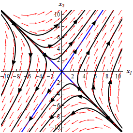
This sketch is called the phase portrait. Usually phase portraits only include the trajectories of the solutions and not any vectors. All of our phase portraits form this point on will only include the trajectories.

In this case it looks like most of the solutions will start away from the equilibrium solution then as \(t\) starts to increase they move in towards the equilibrium solution and then eventually start moving away from the equilibrium solution again.

There seem to be four solutions that have slightly different behaviors. It looks like two of the solutions will start at (or near at least) the equilibrium solution and then move straight away from it while two other solutions start away from the equilibrium solution and then move straight in towards the equilibrium solution.

In these kinds of cases we call the equilibrium point a saddle point and we call the equilibrium point in this case unstable since all but two of the solutions are moving away from it as \(t\) increases.

As we noted earlier this is not generally the way that we will sketch trajectories. All we really need to get the trajectories are the eigenvalues and eigenvectors of the matrix \(A\). We will see how to do this over the next couple of sections as we solve the systems.

Here are a few more phase portraits so you can see some more possible examples. We’ll actually be generating several of these throughout the course of the next couple of sections.

This graph has no domain or range specified.  The horizontal axis is labeled $x_{1}$ and the vertical axis is labeled $x_{2}$.  The graph is labeled “Node – Unstable”. There are two lines with equations of approximately y=x and y=-3/5x on the graph.  Each of these lines have arrow heads on them pointing away from the origin and divide the graph in a giant “X”.  In the upper and right region of the “X” trajectories start at the origin and flow along the y=-3/5x line and at approximately equal distances along the line the break away and flow into the 1st quadrant and move out of the 1st quadrant parallel to the y=x line.  They all have arrow heads on them indicating this direction of motion. In the bottom and left region of the “X” trajectories again start at the origin and flow along the y=-3/5x line and at approximately equal distances along the line the break away and flow into the 3rd quadrant and move out of the 3rd quadrant parallel to the y=x line.  They all have arrow heads on them indicating this direction of motion. This graph has no domain or range specified.  The horizontal axis is labeled $x_{1}$ and the vertical axis is labeled $x_{2}$.  The graph is labeled “Node – Asymptotically Stable”. There are two lines with equations of approximately y=5/3x and y=-x on the graph.  Each of these lines have arrow heads on them pointing towards the origin and divide the graph in a giant “X”.  In the upper and left region of the “X” trajectories start in the 2nd quadrant (for the upper region) and in the 3rd quadrant (for the left region) and flow down and to the right basically parallel to the y=-x line.  As they get near the y=5/3x line they bend in towards that line and follow that line into the origin.  They all have arrow heads on them indicating this direction of motion.  In the upper and right region of the “X” trajectories start in the 1st quadrant (for the right region) and in the 4th quadrant (for the bottom region) and flow up and to the left basically parallel to the y=-x line.  As they get near the y=5/3x line they bend in towards that line and follow that line into the origin.  They all have arrow heads on them indicating this direction of motion.


This graph has no domain or range specified.  The horizontal axis is labeled $x_{1}$ and the vertical axis is labeled $x_{2}$.  The graph is labeled “Improper Node –Unstable”. There is a line with equation of approximately y=-5/3x on the graph with arrow heads on it pointing away from the origin.  Trajectories to the right this line all start at the origin and move away from the origin into the 2nd quadrant.  Trajectories, at approximately equal distances, then bend around and move into the 1st quadrant.  They continue to bend around and move into the 4th quadrant and exit flow out the bottom right corner of the graph basically parallel to the line.  Trajectories to the left this line all start at the origin and move away from the origin into the 4th quadrant.  Trajectories, at approximately equal distances, then bend around and move into the 3rd quadrant.  They continue to bend around and move into the 2nd quadrant and exit flow out the upper left corner of the graph basically parallel to the line. This graph has no domain or range specified.  The horizontal axis is labeled $x_{1}$ and the vertical axis is labeled $x_{2}$.  The graph is labeled “Improper Node – Asymptotically Stable”.  There is a line with equation of approximately y=-3/5x on the graph with arrow heads on it pointing into the origin.  Trajectories above this line all start at the upper part of the graph (in the 1st and 2nd quadrant) and flow down and to the right.  Those that start near the y=-3/5x line in the 2nd quadrant are nearly parallel to the line.  As trajectories move into the 1st quadrant they are not quite parallel to the line.  As the trajectories near the $x_{1}$ axis they bend around and move into the 4th quadrant and start to follow the line into the origin.  Trajectories below this line all start at the lower part of the graph (in the 3rd and 4th quadrant) and flow up and to the left.  Those that start near the y=-3/5x line in the 2nd quadrant are nearly parallel to the line.  As trajectories move into the 3rd quadrant they are not quite parallel to the line.  As the trajectories near the $x_{1}$ axis they bend around and move into the 2nd quadrant and start to follow the line into the origin.


This graph has no domain or range specified.  The horizontal axis is labeled $x_{1}$ and the vertical axis is labeled $x_{2}$.  The graph is labeled “Saddle Point –Unstable”.  There are two lines with equations of approximately y=2/3x (with arrow heads pointing away from the origin) and y=-x (with arrow heads point towards the origin) on the graph. The lines divide the graph in a giant “X”.  In the upper and left region of the “X” trajectories start in the 2nd quadrant and flow down basically parallel to the y=-x line.  As they near the y=2/3x line the bend to the right (for those in the upper region) and to the left (for those in the left region) and follow the y=2/3x line out away from the origin.  Arrow heads are on the trajectories indicating this direction.  In the lower and right region of the “X” trajectories start in the 1st quadrant and flow up basically parallel to the y=-x line.  As they near the y=2/3x line the bend to the right (for those in the right region) and to the left (for those in the bottom region) and follow the y=2/3x line out away from the origin.  Arrow heads are on the trajectories indicating this direction. This graph has no domain or range specified.  The horizontal axis is labeled $x_{1}$ and the vertical axis is labeled $x_{2}$.  The graph is labeled “Center –Stable”.  The trajectories in this graph are three ellipses that are centered on the origin and “angled” so that their major axis (i.e. the long part of the ellipse) are in the 1st and 3rd quadrants.  There are arrow heads on the ellipses indicating they are traced out in a counter clockwise direction.


This graph has no domain or range specified.  The horizontal axis is labeled $x_{1}$ and the vertical axis is labeled $x_{2}$.  The graph is labeled “Spiral –Unstable”.  There are two trajectories on this graph.  Each is a spiral that starts at the origin and rotates out away from the origin  in a counter clockwise manner.  This graph has no domain or range specified.  The horizontal axis is labeled $x_{1}$ and the vertical axis is labeled $x_{2}$.  The graph is labeled “Spiral –Unstable”.  There are two trajectories on this graph.  Each is a spiral that starts at the outer edges (one starts at upper right corner and the other starts at the bottom left corner) and rotates into the origin in a clockwise manner.

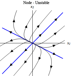
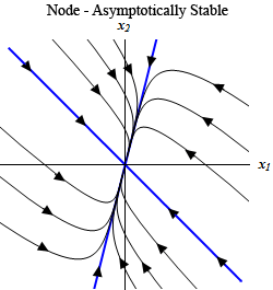
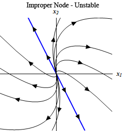
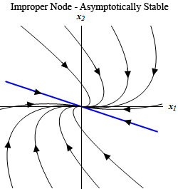
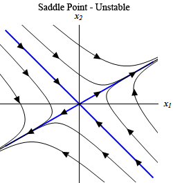
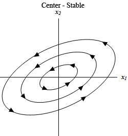
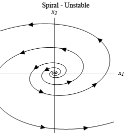
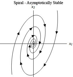
Not all possible phase portraits have been shown here. These are here to show you some of the possibilities. Make sure to notice that several kinds can be either asymptotically stable or unstable depending upon the direction of the arrows.

Notice the difference between stable and asymptotically stable. In an asymptotically stable node or spiral all the trajectories will move in towards the equilibrium point as t increases, whereas a center (which is always stable) trajectory will just move around the equilibrium point but never actually move in towards it.